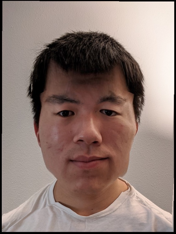
By Adam Chang
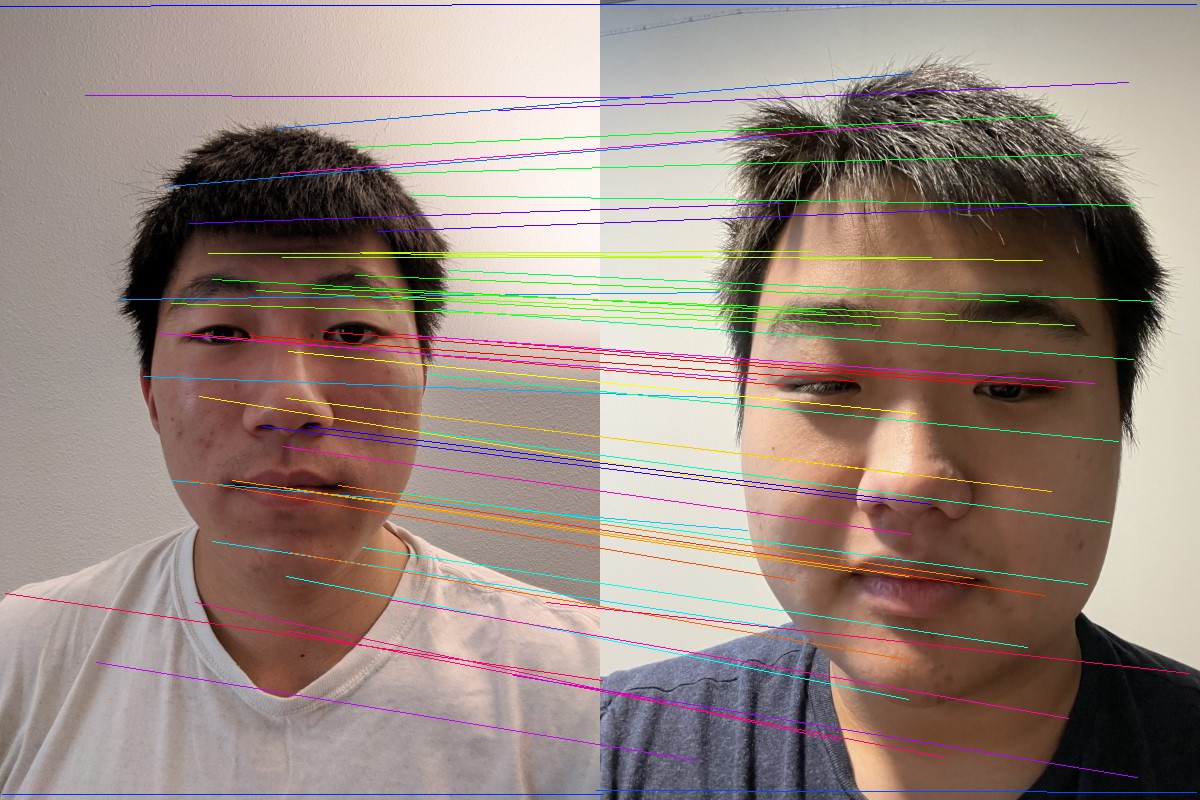
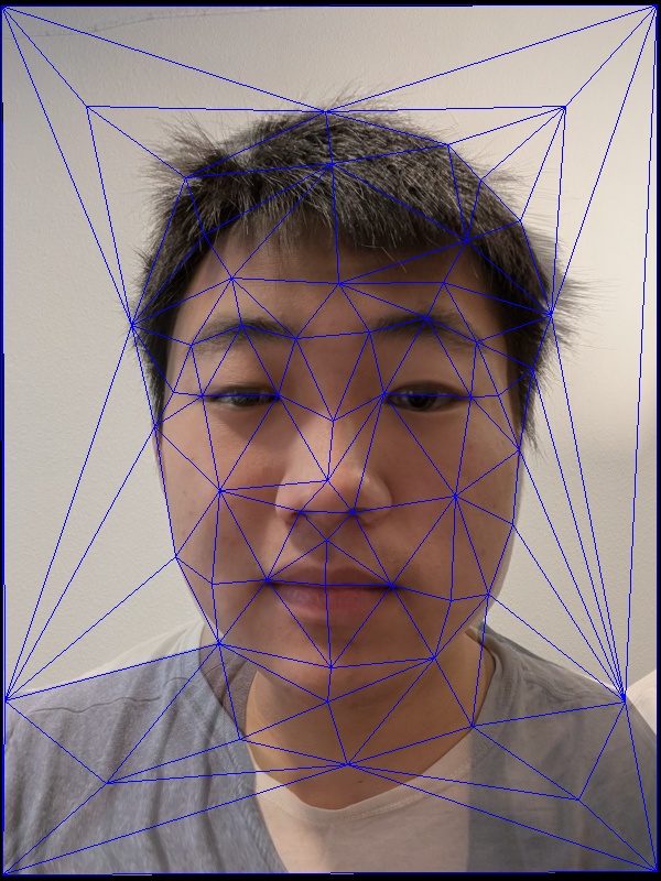
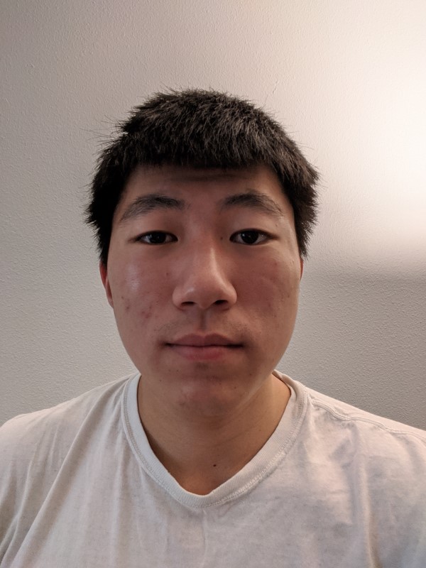
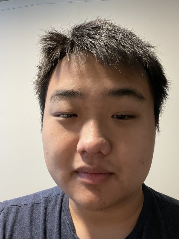
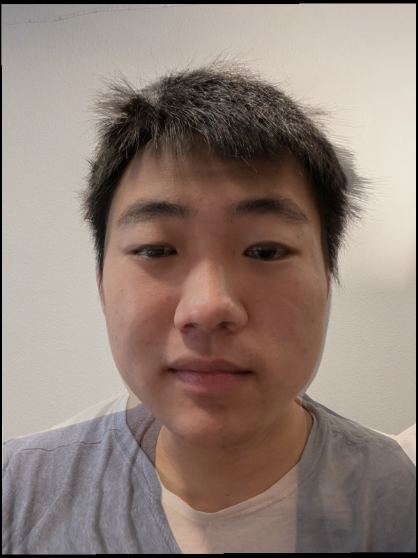
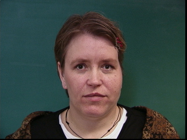
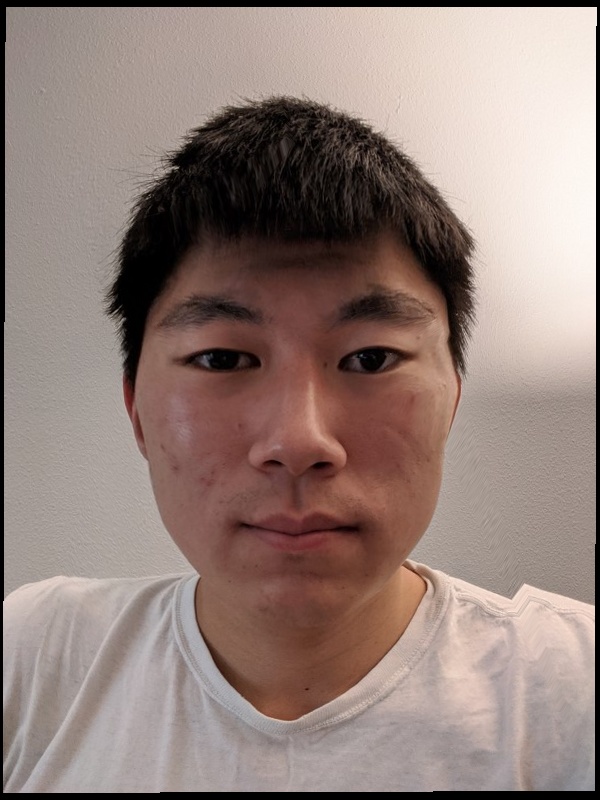
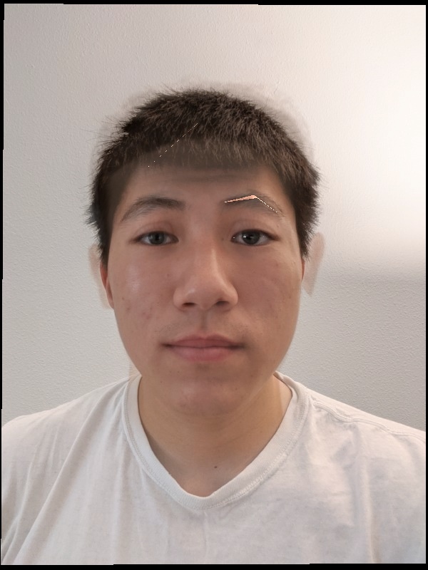
In the first part of the project, we write some of the functionality underlying all the other parts of the project. We begin by writing an interface to manually select keypoint correspondences between two different faces in two different images. This is implemented using [matplotlib.pyplot] to visualize the images and [ginput] to grab pixel coordinates based on where the user clicks. After obtaining these keypoints correspondences between two separate images, we perform triangulation on a set of a keypoints, creating triangles that evenly divide the keypoints in the image into a triangle mesh of adjacent keypoints. This is implemented using [scipy.spatial]'s [Delaunay] algorithm implementation. Below are visualized the manually annotated keypoint correspondences between my face and my friend's face, as well as a triangulation upon the midway face computed in the next part.
In the second part of the project, we perform the morph operation described in class. This involves the following operations:
|
|
|
In the next part of the project, we visualize a morph between two faces. In order to do this, we perform morphing of different amounts between two images. We perform morphing at regular intervals, then display them in increasing order for 1 frame. If we create 60 intermediate images with equal morphing distance, we can generate a 2 second GIF that smoothly transitions two faces.

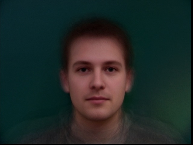
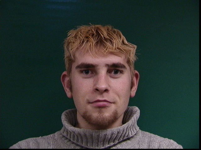
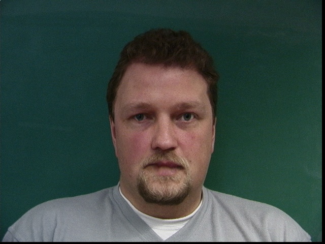
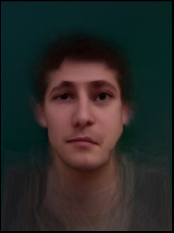
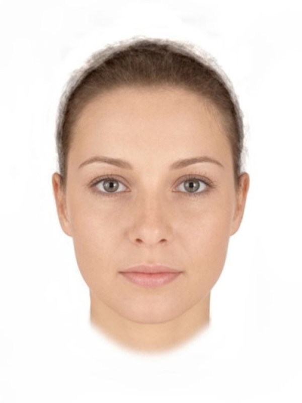
We can apply the techniques used in the morphing part of the project to calculate the average face of an entire population dataset. We can find the average keypoint locations by averaging over all the corresponding keypoint in every face. We can then morph every face to this average structure, and contribute 1/N to the pixel intensities (where N is the size of our dataset). We visualize several results below using the Danes dataset. We see that morphing individual faces to the average structure moves facial features around in order to place them in the most average location. It also shrinks and expands certain facial features to match the average size.
|
|
|
|
|
|
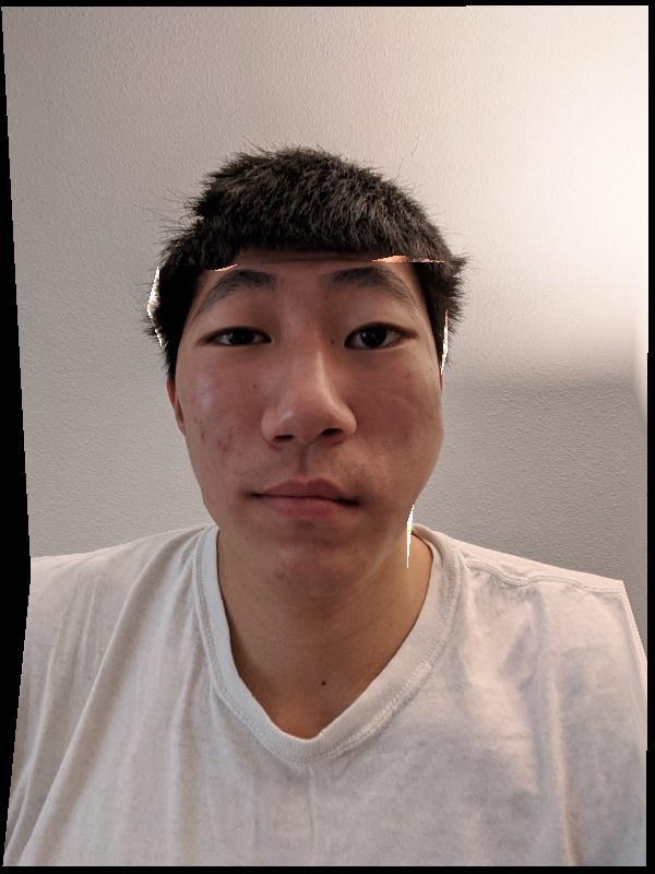
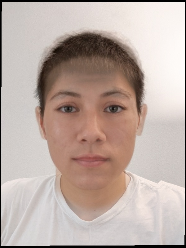
One thing we can do once we have established keypoint correspondences between a face and the average face is to caricaturize the face. This means to exaggerate the aspects of the individual which differ from the average. In terms of position, facial features which are in a different position than the average become even further distanced from the average. Facial features which are larger or smaller than the average become even larger or smaller, respectively. In terms of my face, we can see from the caricature that my right eye is smaller than my left eye, this imbalance is exaggerated in the caricature. Additionally, my forehead is smaller than the average, and now it is even more so.
By obtaining different subpopulation averages, we can perform other operations on an individual face. For example, in this part, I morph my face with the average female face. First, we only morph the structure. Next, we only morph the appearance. Finally, we morph both.
|
|
|
|
|
|