Project 3 Report

1 Defining Correspondence

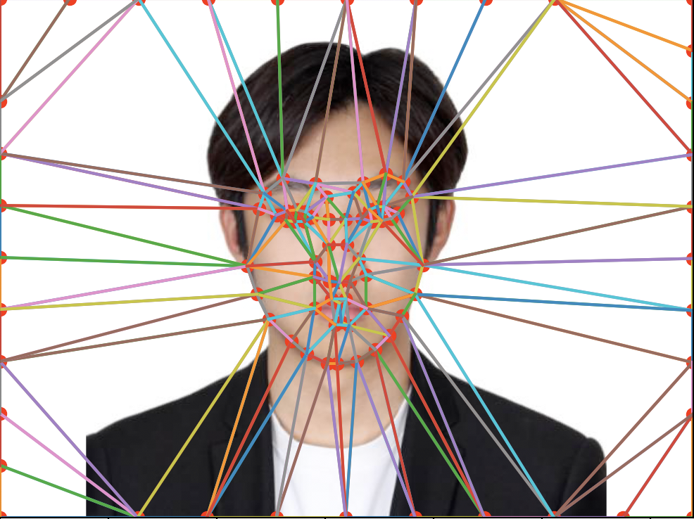
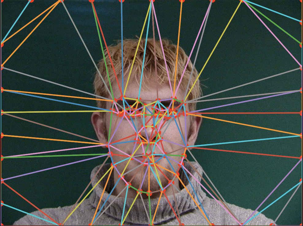
For this assignment, I used the Imm Dataset (https://web.archive.org/web/20210305094647/http://www2.imm.dtu.dk/~aam/datasets/datasets.html) and followed their annotation format. The illustration of a sample image of the dataset and a photo of mine is shown below. Both are annotated and triangulated in the same form. Further, I added border keypoints of the image such that morphing the face will not greatly morph the other areas. Triangulation is constructed via Delaunay's algorithm.

2 Mid-way Face

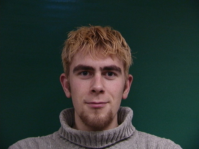
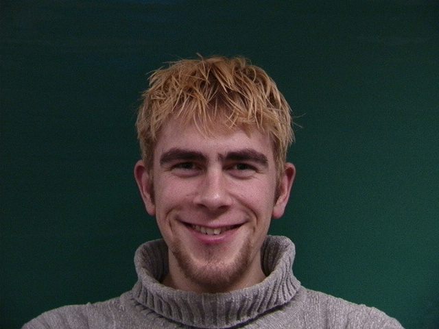
First, The average shape is computed as the average of the two point sets. Then, I created a new canvas of the same size as the input images which is used to paint the midface. To map the pixels onto the canvas, I used inverse affine transformation for each pair of triangles. Concretely, for each pixel in a certain average shape triangle, its corresponding pixel in the original image is computed by inverse affine transformation. If the corresponding pixel is at a non-integer position, then bilinear interpolation is used to calculate its pixel value. Then the value is copied onto the canvas. The final midface is the average the two input images mapping onto the canvas. The mid-way face of the same person smiling and not smiling in the Imm Dataset is shown below.

3 The Morph Sequence

Constructing a morph sequence is much similar to constructing the midface instead the target shape is not the average the two input images, but a weighted average of the two with the weight changes by time. Let's define two weights, warp fraction and dissolve fraction. For each frame, it can be generated by a function with its interface definition like

        morph_image_pairs(img1, img2, pts1, pts2, tri, warp_frac, dissolve_frac)
    

4 Mean Face of a Population

This is also much similar to computing the mid face. First, the average shape is computed over all the images in Imm Dataset. For each image, the pixels are mapped to the canvas via inverse affine transformation and bilinear interpolation. The final average face is the average canvas. Mean faces of Imm Dataset for smiling/non-smiling, male/female is shown below. (The grayscale images are removed, and only frontal images are reserved.)

Given these meanfaces, I can do a switch between my face and the average face of the dataset. Here, switching only involves the shapes of the two images. The results of switching my face and the meanface of men without smiling is shown below.

However, the above results is somehow over-morphing both images. I found that empirically, using the interface developed in Section 3 by setting warp fraction=0.5 and dissolve fraction=0 produces good results. The results are shown below.

5 Caricature

Using the same interface in Section 3, we can easily extrapolate an image from the population mean. This can be done by setting the warp fraction larger than 1 or smaller than 0. Results are shown below (big caricature: warp fraction=1.5, small caricature: warp fraction=-0.5).

6 Bells & Whistles

6.1 Automatic Morphing

Annotating all the keypoints on a face can be burdensome. We can use some automatic keypoint detection tools to free us from this tedious job! In this assignment, I used face detection and keypoint detection toolkit provided in dlib package. The extracted keypoints and triangulation as well as a morph sequence is shown below. The inputs are photos of my friend now and at the age of 18.

6.2 Morphing across Ethnicity

I collected several mean faces of males of Chinese, Japanese, Korean, African, Italian, and Germany. All of these images are annotated manually in the same format as Imm Dataset. The morph sequence is constructed by only morphing just the shape, the color, and both. First, I define several capstones for the sequence, for example, the capstone for morphing both the shape and color is created by using the interface in Section 3, with warp and dissolve fraction=0.5. For morphing only the shape or the color, it is done by setting dissolve or warp fraction to 0. The following results show the morph sequence from one ethnicity to another. Apparently, morphing using both the shape and color produces much better results.

6.3 Friends Morphing - The Music Video

Technically, the frames are created as in Section 3, but with music. The video is shown below.