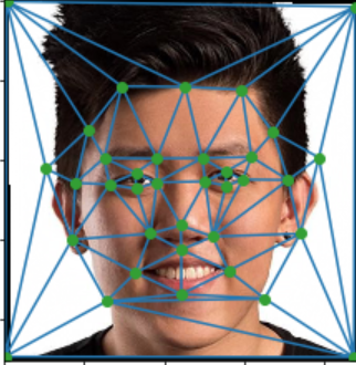
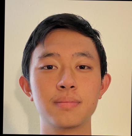
Part 1: Definining Correspondences
The goal of this part is to select pairs of corresponding points on our two images, which will be used to create a triangulation for affine morphing. I used ginput to select the points in a Jupyter notebook. Then, I computed the average of the point sets and used Delauanay triangulation on the average point set.
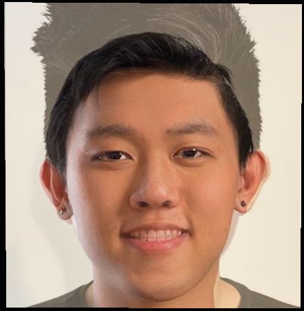
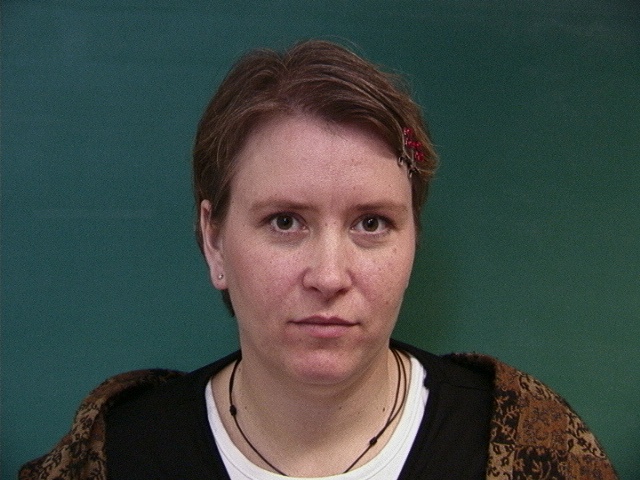
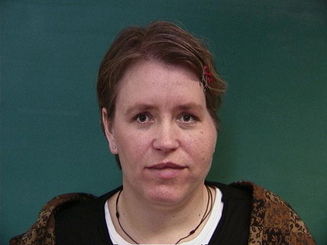
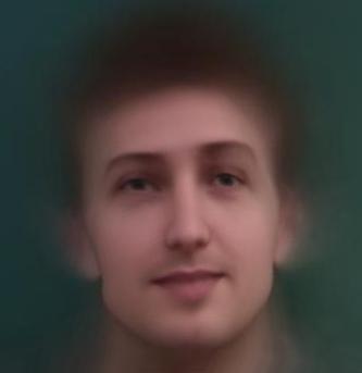
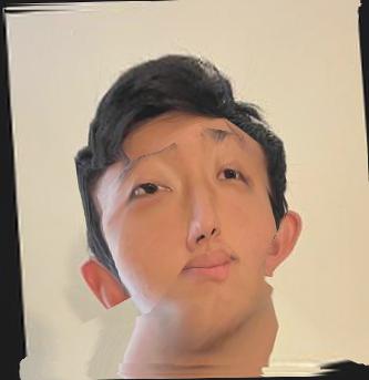
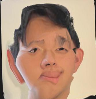
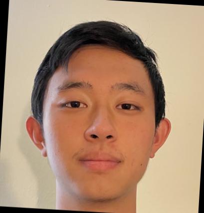
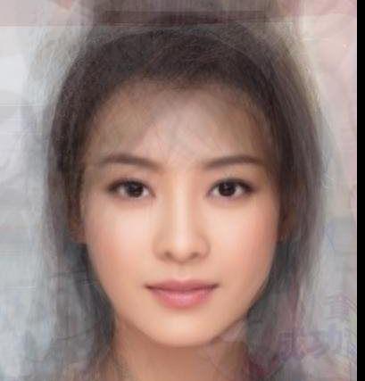
Here are my input images are myself, and TFT streamer C9 k3soju:
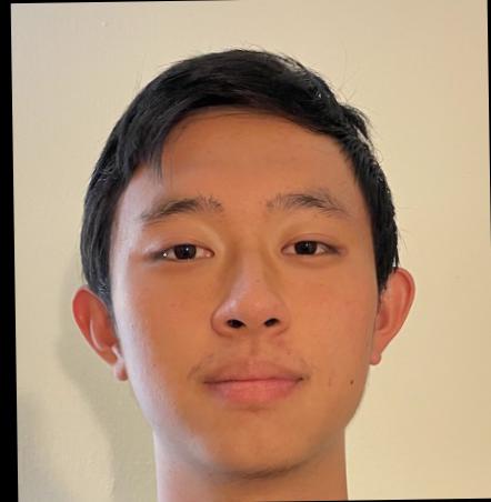
Kevin
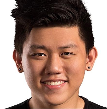
C9 k3soju
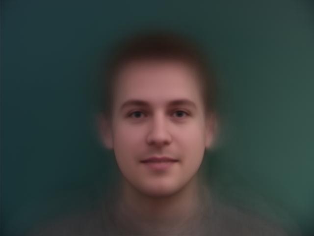
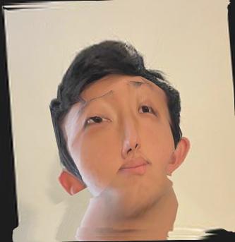
Triangulation Results:
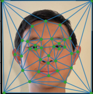
Kevin Triangulation