Overview
In Part A of this project, we aim to compute homographies between image planes and use this to create mosaics.
Part 1: Shoot and Digitize Images
|
|
|
|
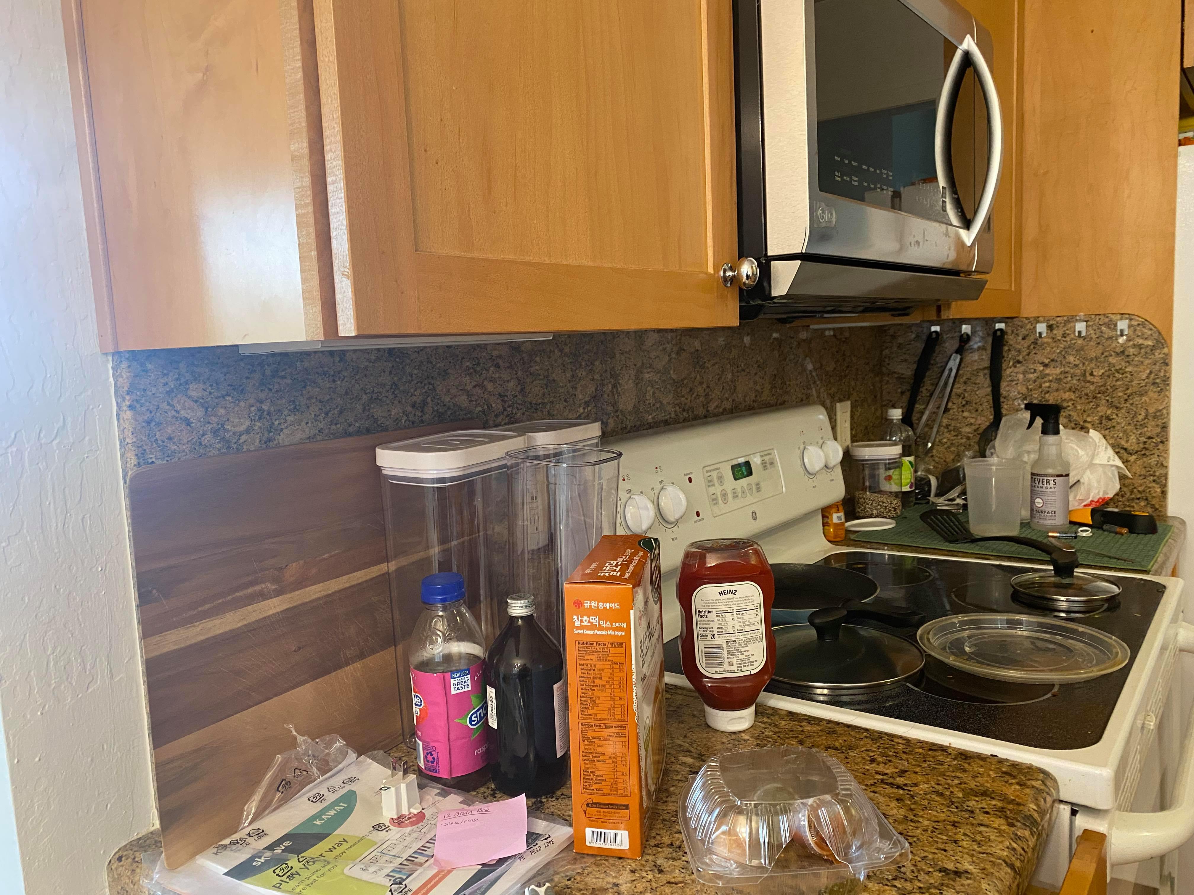
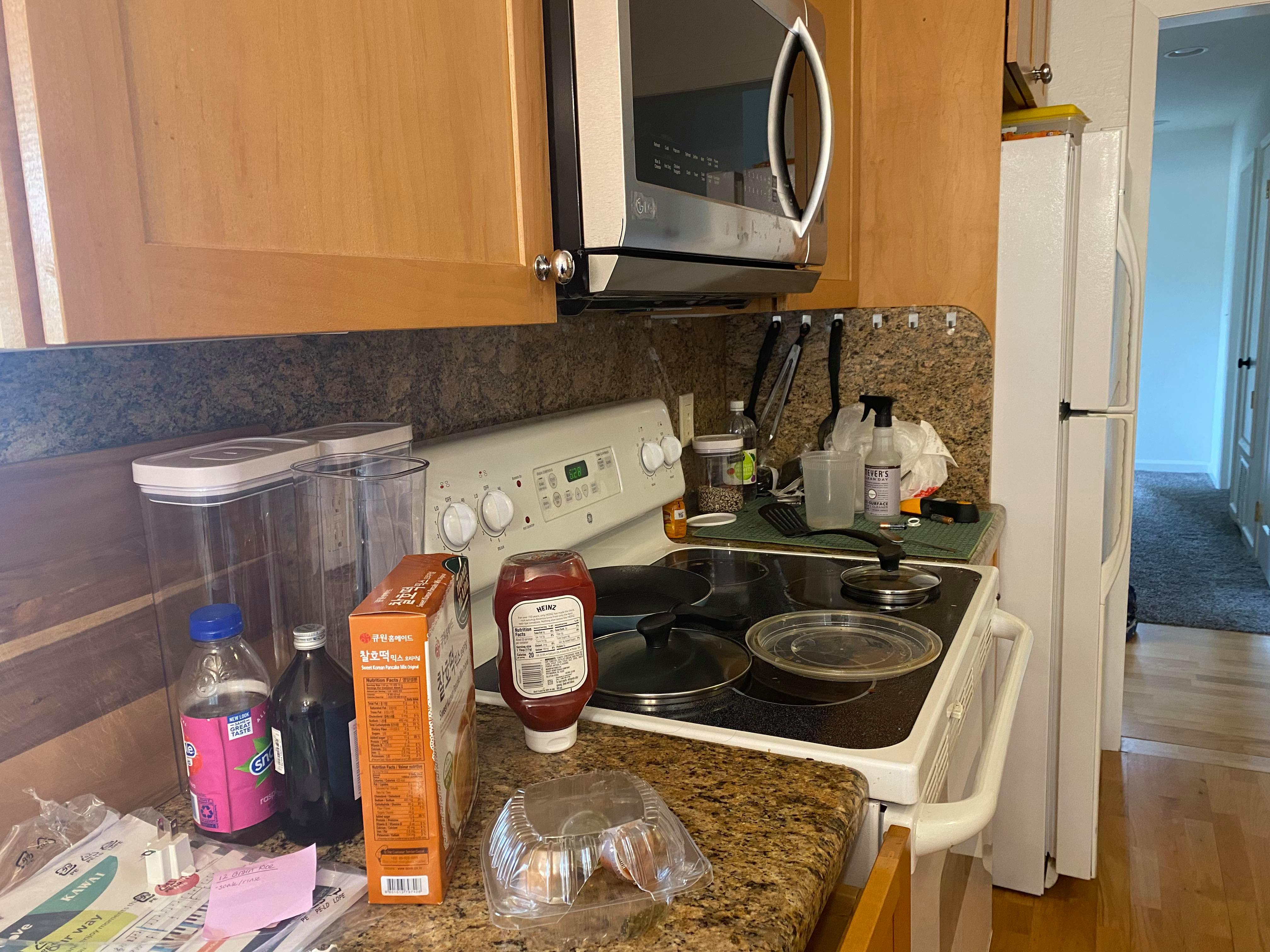
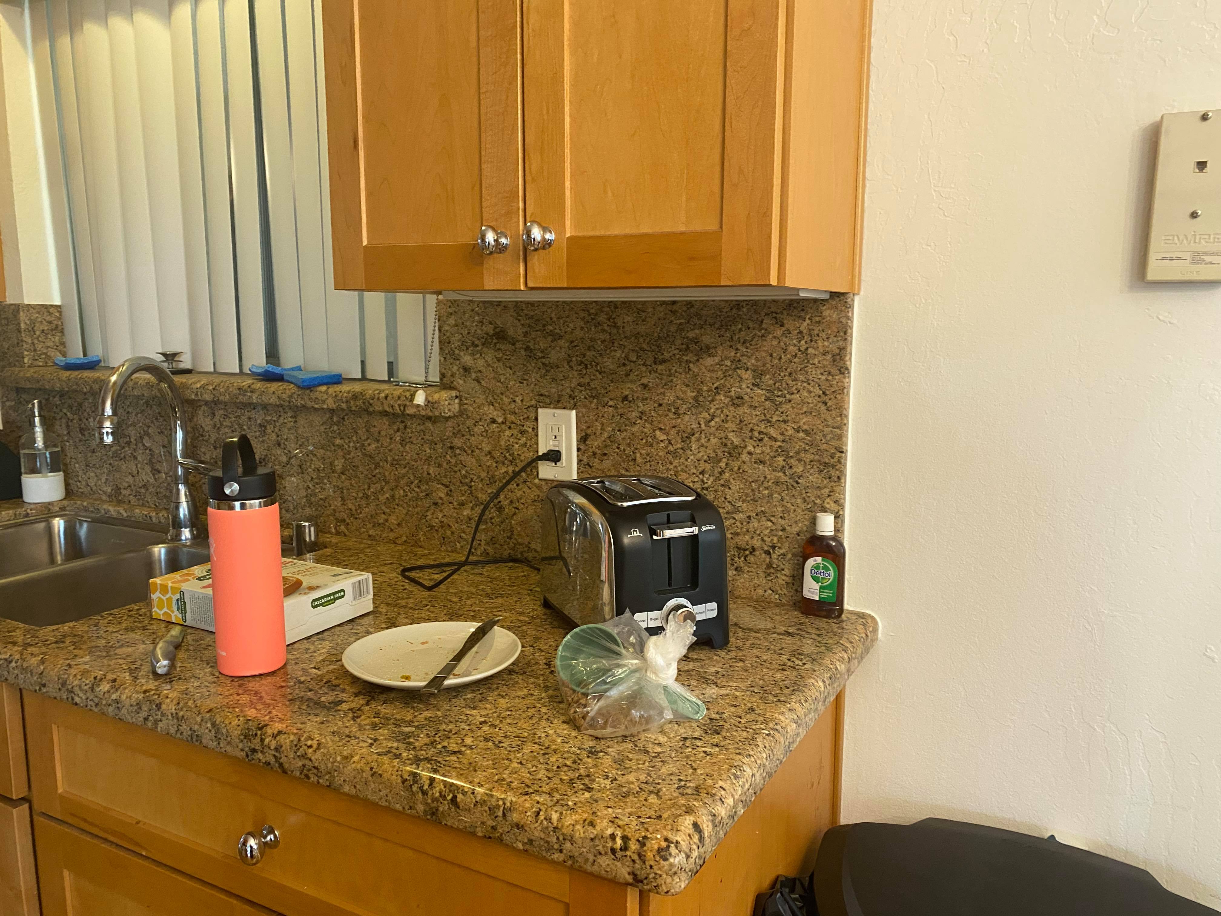
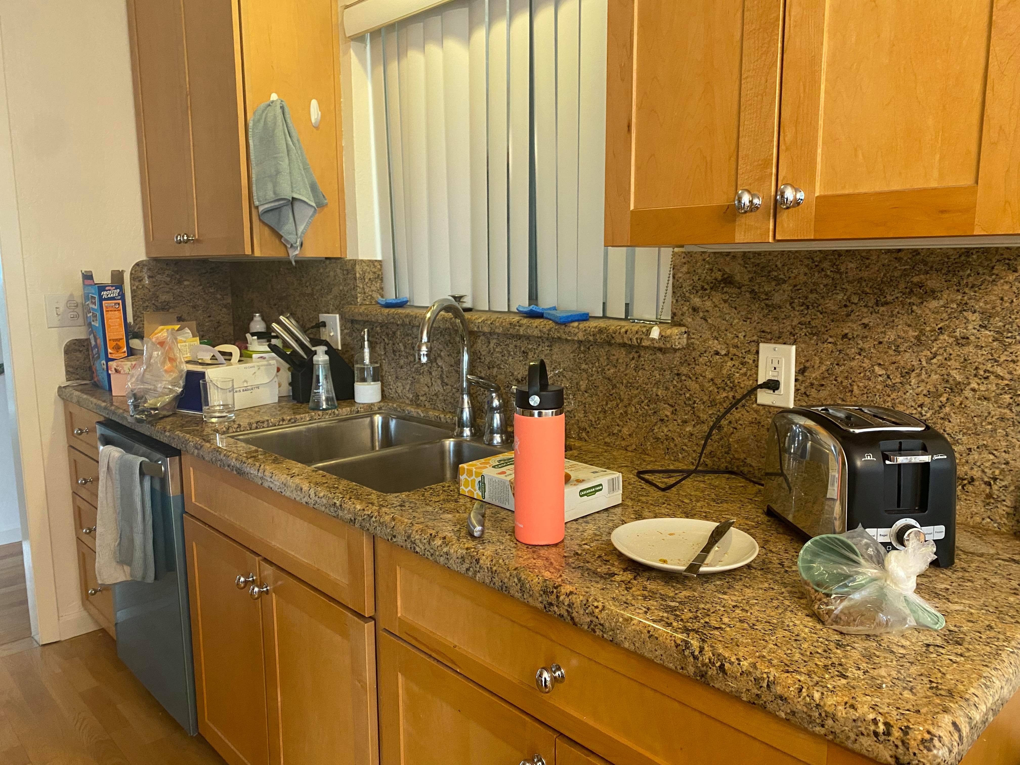
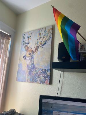
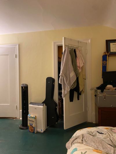
For the following parts of the project to work (particularly the mosaicing), it is important for us to take photos that have the same center of view. For this project, I used my smartphone (iPhone 11) and tried to rotate my body while keeping the camera still. I locked the exposure and focus to make sure the photo looks consistent. The above are the photos for the mosaic. The below are photos used to show image rectification.
|
|
Part 2: Recover Homographies
|
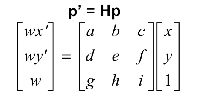
To properly warp the images, we must first recover the homography to do so. Figure 3 shows how the homography is set up. We are looking for the values of H. We know wx', wy', x, and y. wx' and wy' are the target coordinates in a plane. The x, y are the source coordinates from the originaly image. We set i to be 1, and we then try to solve for the remaining 8 parameters a-h.
To do so, we can set up a system of linear equations. We primarily note that wx' = ax + by + c. wy' = dx + ey + f. w = gx + yh + 1. Rearranging all this gives us the following system of equations:
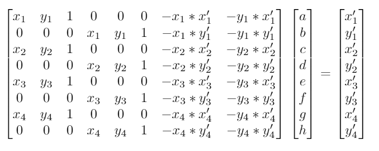
|
Once in this form, we can solve for the entries a-h. However, we can also extend this to be an overparameterized problem. Rather than include only 4 points, we can extend this to any n points instead. This means that the H matrix is n*2 rows by 8 columns. The corresponding b matrix is n*2 rows as well with x and ys alternating. We can solve this with a linear least squares solver such as numpy.linalg.lstsq.
Consequently, we can quite easily define a function computeH(im1_pts, im2_pts). im1_pts contains all the x, y to populate the A matrix. The im2_pts contains the x', y' to populate the b matrix. Then we use linear least squares to solve for elements a-h and use 1 to round out the 9th value. This is our homography matrix.
Part 3: Warp Images
Once we have the homography, we can write some function warpImage(im, H) that warps the image to the desired plane. We use inverse warping. We do the following steps.
- Calculate where all the corners of the image go in the new plane. Use this to calculate the shape of the bounding box for the warped image.
- Calculate where all the internal pixels go. This is actually done with an inverse warp.
- Calculate H_inv
- Multiply H_inv with every pixel in the new image that corresponds to pixels from the source image.
- Now populate the colors properly.
- Generate the RectBivariateSpline functions for each color channel of the image
- Use these functions to inverse warp to get the appropriate colors.
This is very similar to the warping that we did in the previous project.
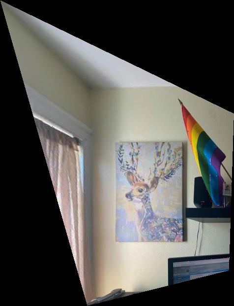
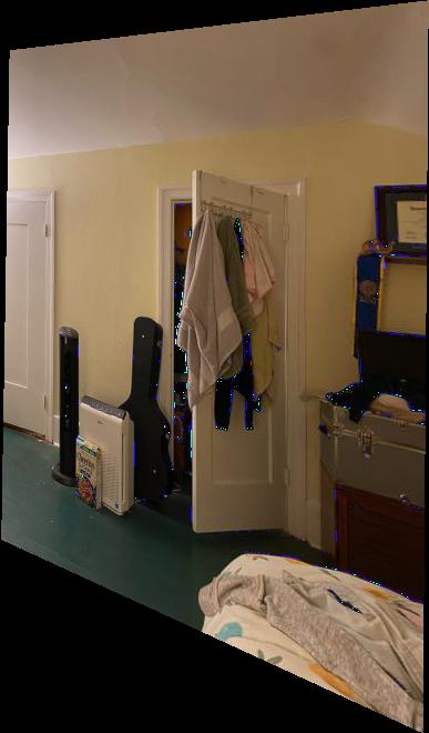
Part 4: Image Rectification
Now that we have the warp, we can "rectify" images. In these examples, we take images of planar surfaces and then warp them so the plane is frontal-parallel. We find the pixels of the corners of our planes, decide where we want them to go in the final image, and then call computeH and imwarped accordingly to generate the following images.
|
|
|
|
|
|
Part 5: Mosaics
Didn't get here yet :(