Project 4 [Auto]Stitching Photo Mosaics

2021 Fall CS 294-026 Xinwei Zhuang

---

Part 1: Image Warping and Mosaicing

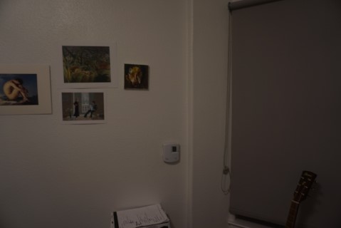
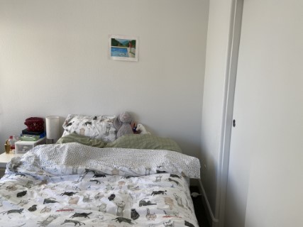
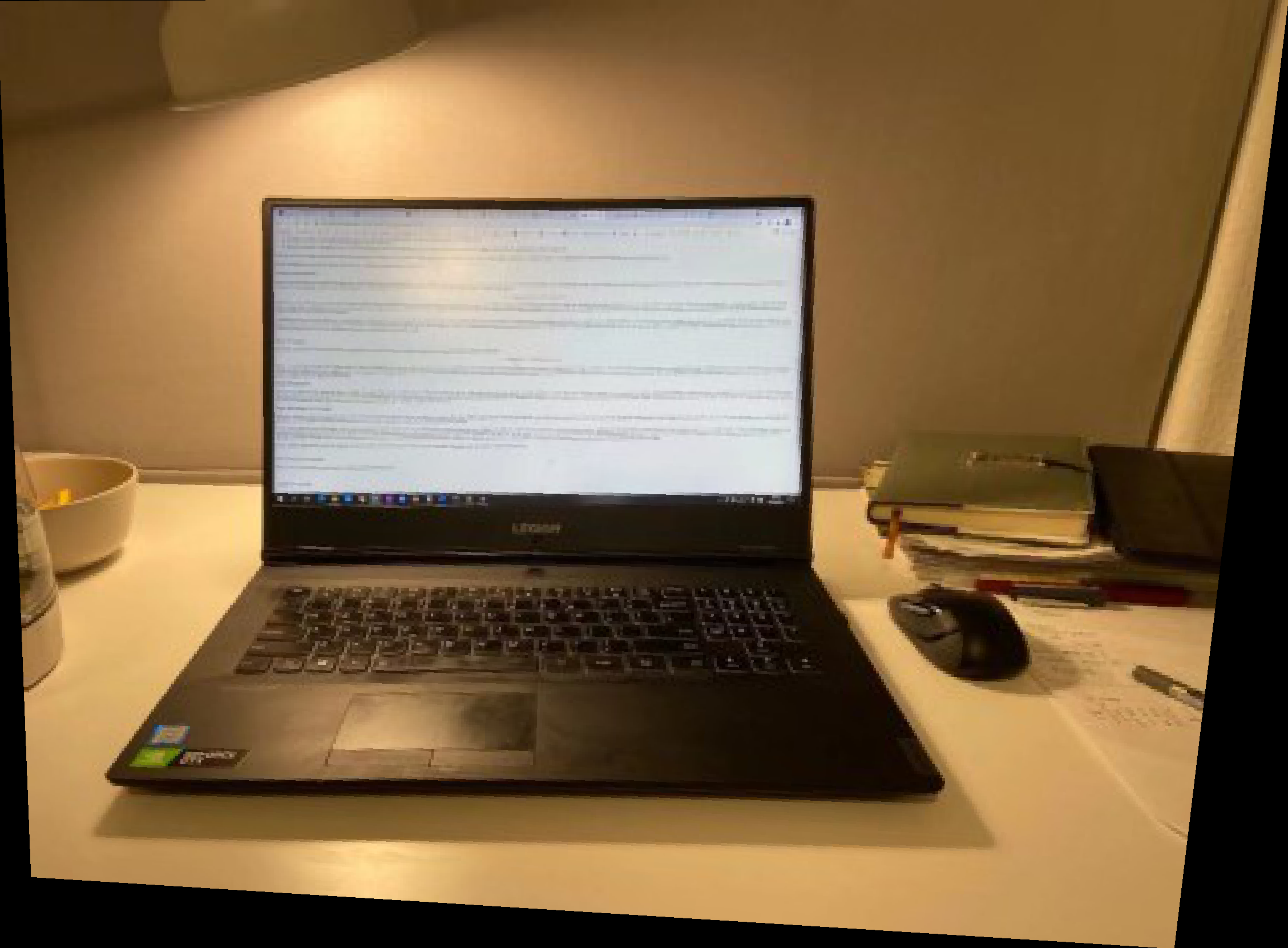
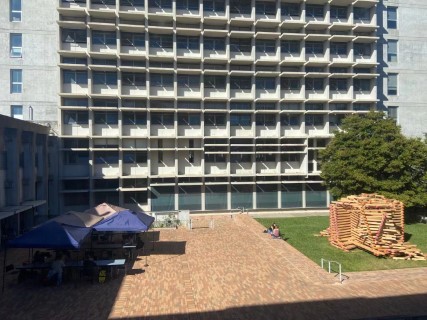
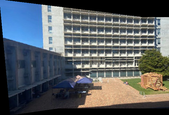
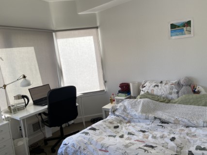
Step 1: Shoot and digitize pictures

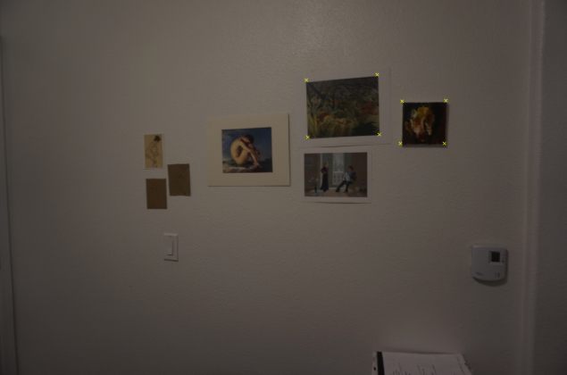
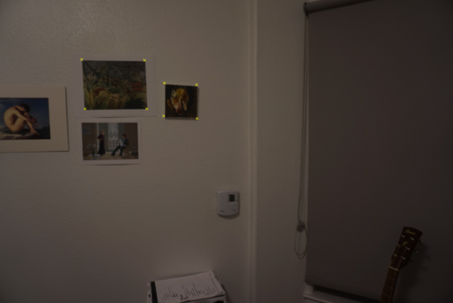
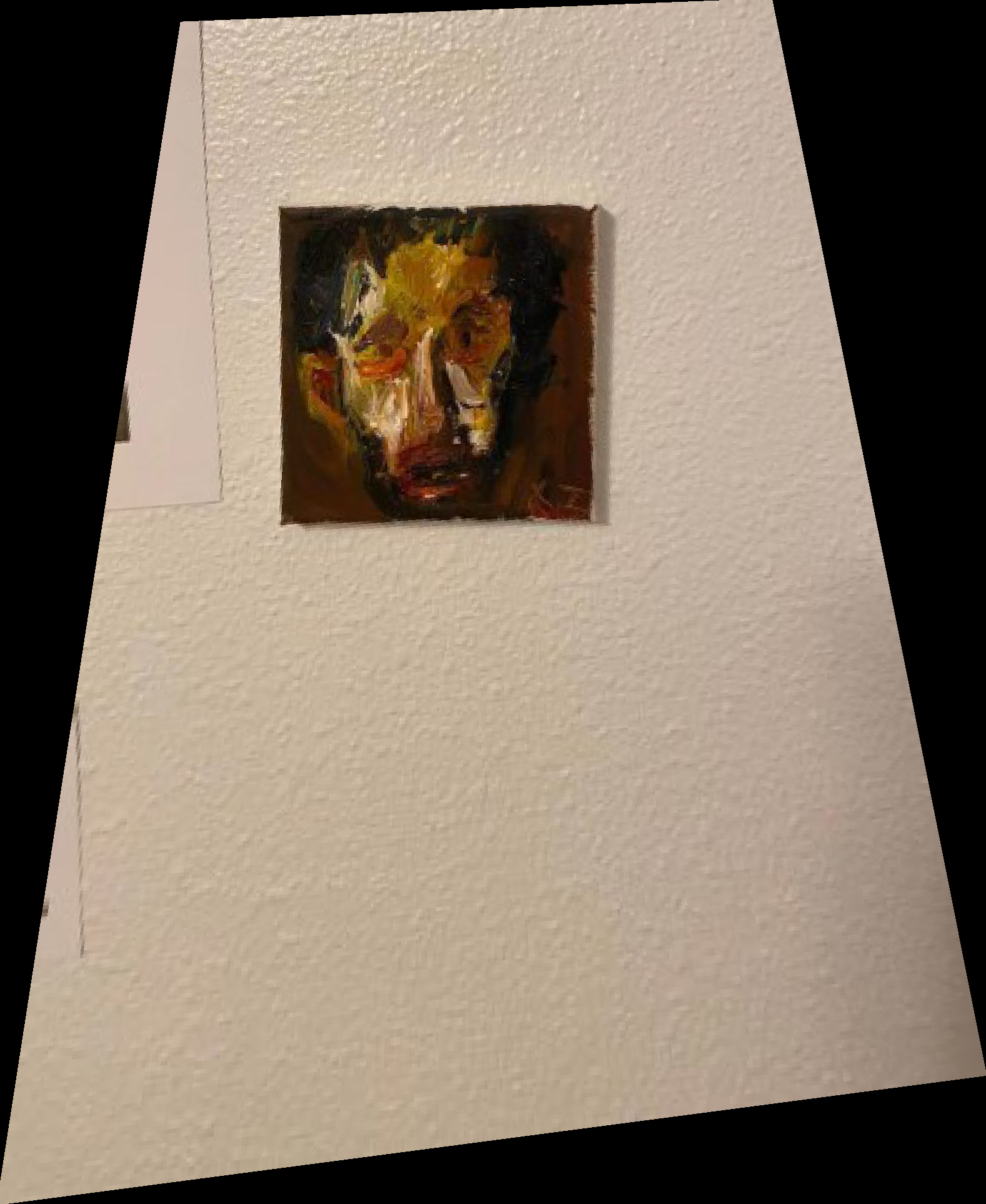
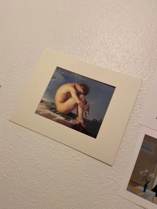
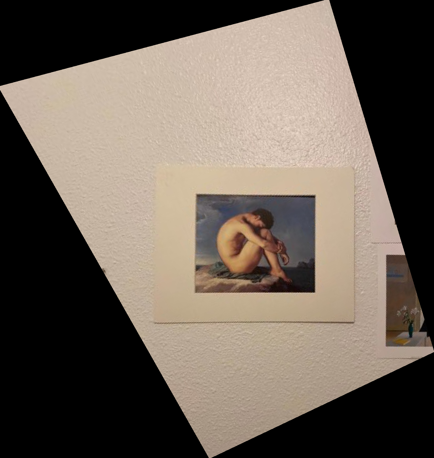
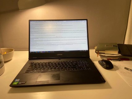
Picture is my bedroom using sony alpha 5000. All parameter is identical, and the camera only rotates but does not move.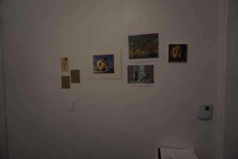

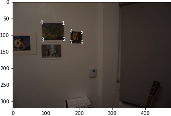
Step 2: Recover homographies

To recover the homographies, a set of corresponding points are manually selected, the selected points are as follows.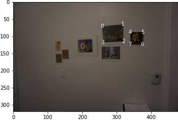 Since they are not accurate to a pixel level, I then need to fine-tune the points to the real pixels. I used normalized-correlation matching from Project 1 to find the accurate points' coordinates. The adjusted coordinates are plot below. The adjusted points are as follows.
Then a Homography matrix is calculated by p'=Hp. There are 8 unkown variables. With 4 points (8 equations), the system will provide a result. In this case, 8 points will provide a overdetermined result. To get the warped pixels, the equation for transforamtion is: $$ \begin{bmatrix} wx' \\\ wy' \\\ w \end{bmatrix} = \begin{bmatrix} a & b & c \\\ d & e & f \\\ g & h & i \end{bmatrix} \begin{bmatrix} x \\\ y \\\ 1 \end{bmatrix} $$ Since one image only shares a single scale factor $w$, we can expand the equation above into the following format: $$ \begin{bmatrix} x_1 & y_1 & 1 & 0 & 0 & 0 & -x_1'\cdot x_1 & -x_1' \cdot y_1 \\\ 0 & 0 & 0 & x_1 & y_1 & 1 & -y_1'\cdot x_1 & -y_1' \cdot y_1 \\\ x_2 & y_2 & 1 & 0 & 0 & 0 & -x_2'\cdot x_2 & -x_2' \cdot y_2 \\\ 0 & 0 & 0 & x_2 & y_2 & 1 & -y_2'\cdot x_2 & -y_2' \cdot y_2 \\\ \vdots\\\ x_n & y_n & 1 & 0 & 0 & 0 & -x_n'\cdot x_n & -x_n' \cdot y_2 \\\ 0 & 0 & 0 & x_n & y_n & 1 & -y_n'\cdot x_n & -y_n' \cdot y_2 \end{bmatrix} \begin{bmatrix} h_{11} \\\ h_{12} \\\ h_{13} \\\ h_{21} \\\ h_{22} \\\ h_{23} \\\ h_{31} \\\ h_{32} \end{bmatrix} = \begin{bmatrix} x_1' \\\ y_1' \\\ x_2' \\\ y_2' \\\ \vdots \\\ x_n' \\\ y_n' \end{bmatrix} $$ To solve the homographies, more than 4 points are needed, so we have at least 8 equations to solve Homography matrix. In this project, 8 points are used for each pair of photos. Thus 16 equations is used to solve a homography matrix. The above equation is then translated and a constraint $|H|=1$ is added to avoid H being all zeros. $$ \begin{bmatrix} x_1 & y_1 & 1 & 0 & 0 & 0 & -x_1'\cdot x_1 & -x_1' \cdot y_1 & -x_1'\\\ 0 & 0 & 0 & x_1 & y_1 & 1 & -y_1'\cdot x_1 & -y_1' \cdot y_1 & -y_1'\\\ x_2 & y_2 & 1 & 0 & 0 & 0 & -x_2'\cdot x_2 & -x_2' \cdot y_2 &-x_2'\\\ 0 & 0 & 0 & x_2 & y_2 & 1 & -y_2'\cdot x_2 & -y_2' \cdot y_2 &-y_2'\\\ \vdots\\\ x_n & y_n & 1 & 0 & 0 & 0 & -x_n'\cdot x_n & -x_n' \cdot y_2 & -x_n'\\\ 0 & 0 & 0 & x_n & y_n & 1 & -y_n'\cdot x_n & -y_n' \cdot y_2 & -y_n'\\\ 0 & 0 & 0 & 0 & 0 & 0 & 0 & 0 & 1 \end{bmatrix} \begin{bmatrix} h_{11} \\\ h_{12} \\\ h_{13} \\\ h_{21} \\\ h_{22} \\\ h_{23} \\\ h_{31} \\\ h_{32} \\\ h_{33} \end{bmatrix} = \begin{bmatrix} 0 \\\ 0 \\\ 0 \\\ 0 \\\ \vdots \\\ 0 \\\ 0 \\\ 1 \end{bmatrix} $$ Finally, SVD is used and the last singular vector V is selected as the solution of H.

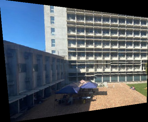
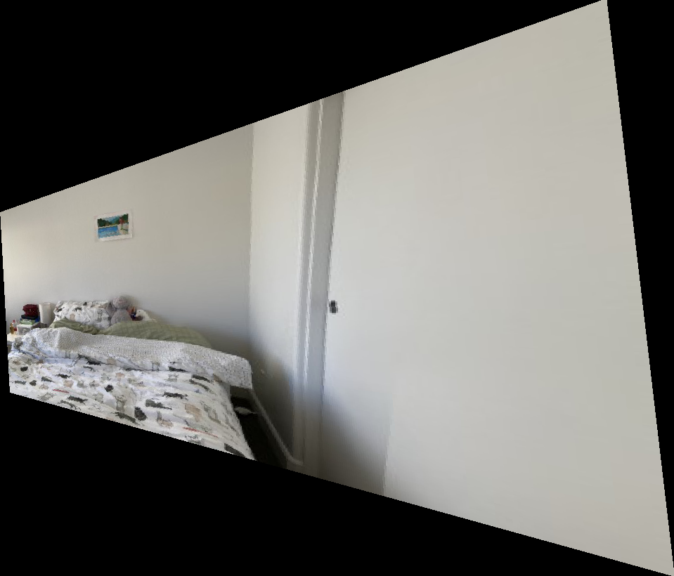
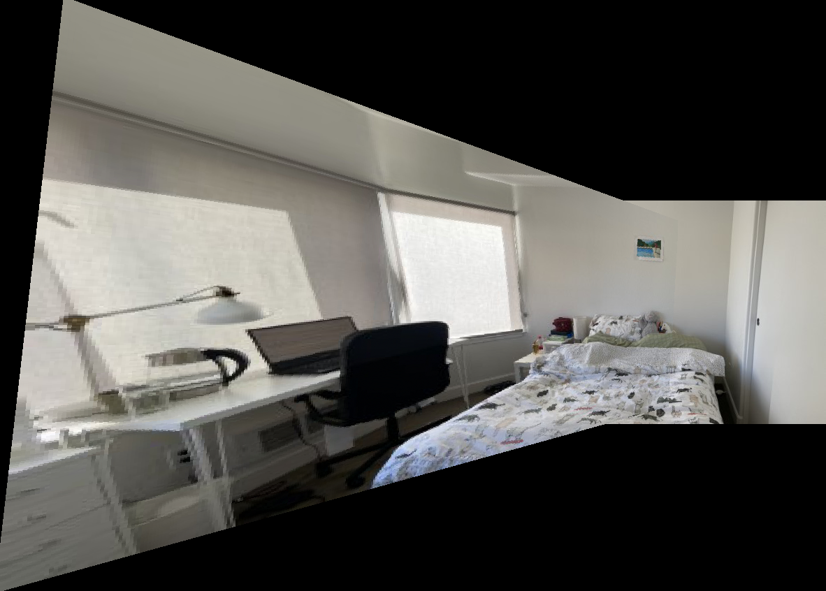
Step 3: Warp the images (Image Rectification)

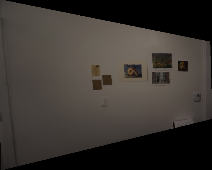
An inverse warping is used to find corresponding points. Interp2D is used for antialias. Results of warping image 1 into the plane of image 2 is shown below.
With homography matrix, I can morph any image with planary identity to its non-distorted view. Several examples are shown below.

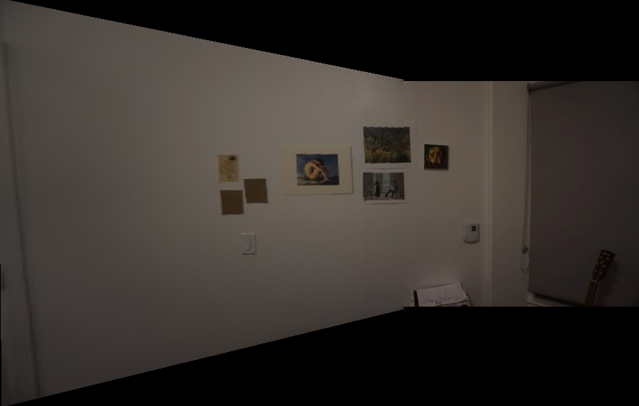
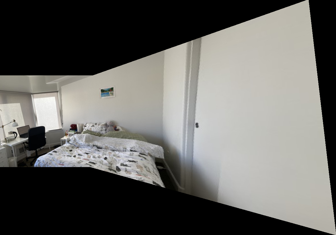
Step 4: Blend images into a mosaic

To blend images, first step is to find the canvas size, then add pixels from the original images to target position with a alpha mask. The results on 3 sets of images are shown below. (Sorry for the boing results!) Result image

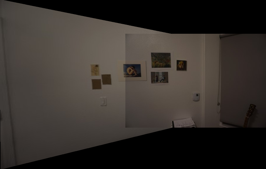
Though it looks not bad, Notice that the colour is not same between two images. One is cooler and one is warmer. To provide a more smooth transicent, a weighted averaging mask is performed. The resulting blending after applying a Laplacian pyramid blending is shown below. The edge is nearly invisible now. :)

Result image

Result image (for these photos I tried to morphy them with different target images. Both are not satisfying, changing them to cylinder projection will probably behave better.)

Step 5: Bells and Whistles

For the bedroom photo mosiac. I project the photos back on a cylinder screen to see whether it will provide a less artificial looking image.

What I've learnt

The homography matrix is dependent on the quality of the feature points. Firstly it took me too long to find a satisfying morphing, but I realised that this is due to the inaccurate feature points. I turned to Matlab for auto fine tuning the feature points and the transformation gets better.

For image blending, there are a lot of tricks that can make the blending better. I just used one of the naive one, a weighted averaging to feather the edges. If more clarity is required, a Laplacian pyramid blending can also be used for ghosting of high-frequency terms.

The projected image can look badly artificial if the projection method is not chosen carefully. For rotated photos, the morphed image looks better when project onto a cylinder screen.

Part 2: Feature Matching for Autostitching

Step 1: Detecting corner features in an image

Step 2: Extracting Feature Descriptor

Step 3: Matching feature descriptors

Step 4: Robust method (RANSAC) to compute homography

Step 5: Image mosaic

Bells & Whistles

Reference

For homography matrix:
https://math.stackexchange.com/questions/494238/how-to-compute-homography-matrix-h-from-corresponding-points-2d-2d-planar-homog

For Harris corner feature detection
Brown, M., Szeliski, R., & Winder, S. (2005, June). Multi-image matching using multi-scale oriented patches. In 2005 IEEE Computer Society Conference on Computer Vision and Pattern Recognition (CVPR'05) (Vol. 1, pp. 510-517). IEEE.