Image Warping and Mosaicing Part A
CS 194-26 Image Manipulation and Computational Photography – Project 4A, Fall 2021
Adnaan Sachidanandan
Shoot the Pictures
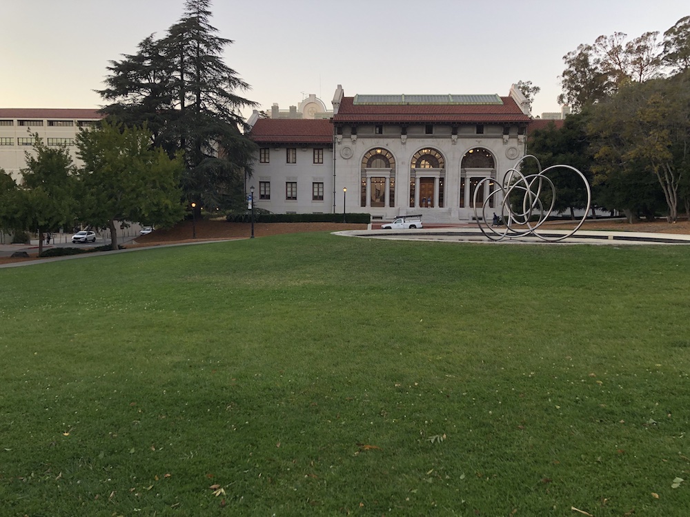
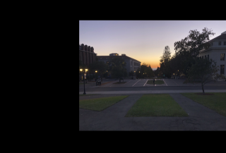
To begin, I went around Berkeley's campus taking pictures with around 50% overlap to warp and mosaic together. Each picture was taken on my phone with the exposure and focus locked
between each angle. The original images are displayed below:
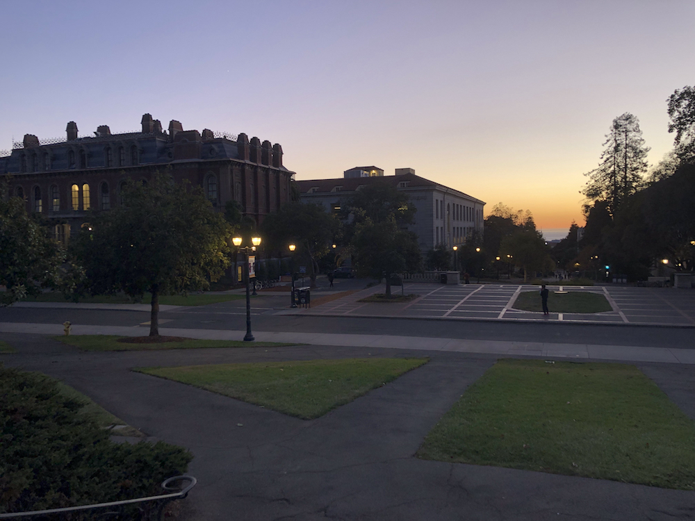 Campanile Way Dusk - Left
|
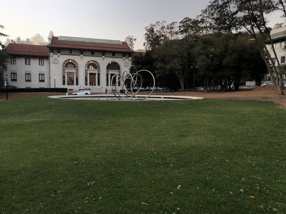
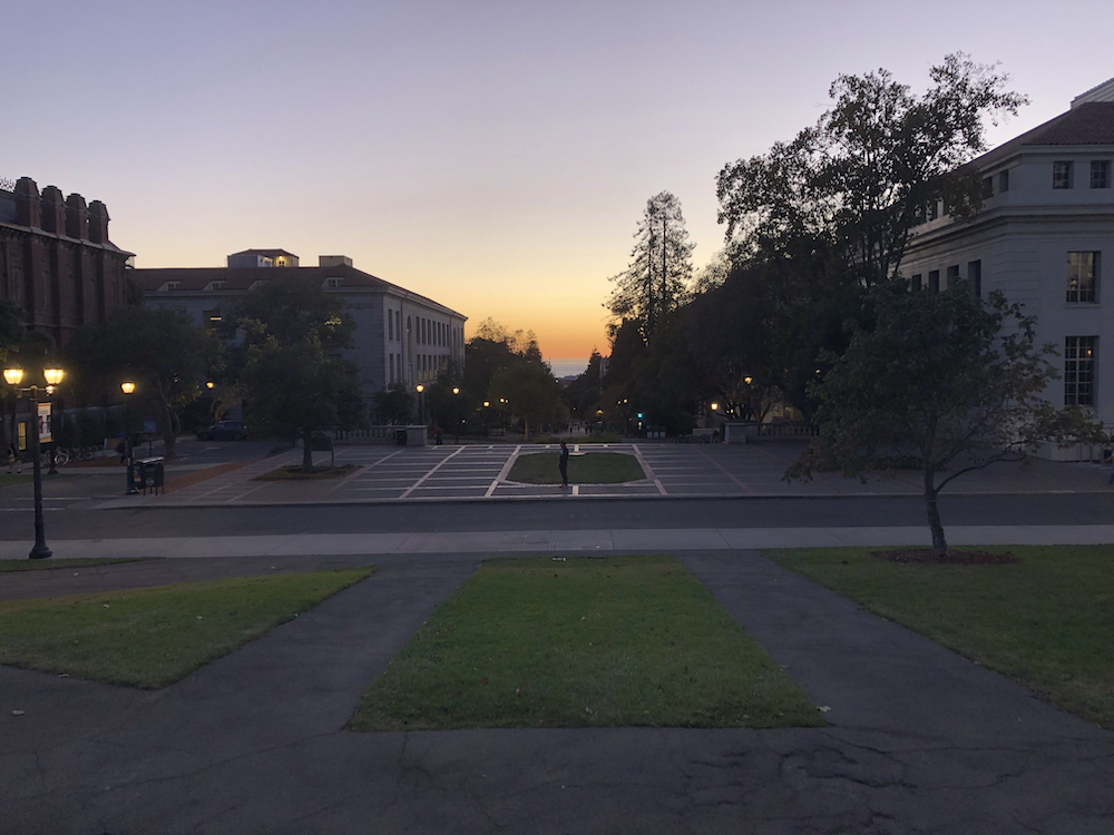 Campanile Way Dusk - Center
|
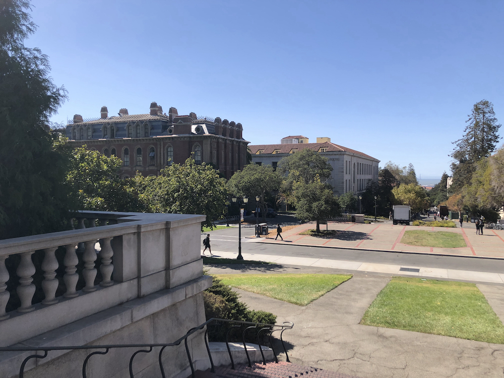 Campanile Way Day - Left
|
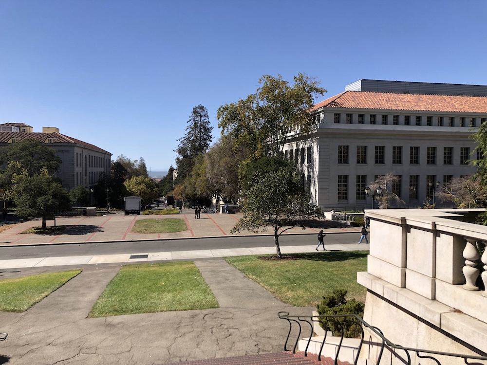 Campanile Way Day - Right
|
 Hearst Mining Circle - Left
|
 Hearst Mining Circle - Right
|
Recover Homographies
With the pictures, we need to figure out the perspective transformation that brings us from one image to the other. The perspective transform we need to recover is the following matrix H where p is the correspondence points from
one image and p' is the equivalent correspondence points from the other image:
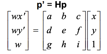 Since H has 8 degrees of freedom (we set i to be 1), we need at least 8 correspondence equations to figure out the other parts of the homography matrix. Since each point in an image has two coordinates,
this means we need 4 points from one image and their corresponding points in the other image, giving us 8 equations (one equation for each mapped x and one for each mapped y). Then, with these points we can
use least squares to estimate the parameters for the homography matrix, H. In my implementation more specifically, I created Eq. (13) from this helpful explanation
on estimating homographies, and used least squares to get the h vector.
Since H has 8 degrees of freedom (we set i to be 1), we need at least 8 correspondence equations to figure out the other parts of the homography matrix. Since each point in an image has two coordinates,
this means we need 4 points from one image and their corresponding points in the other image, giving us 8 equations (one equation for each mapped x and one for each mapped y). Then, with these points we can
use least squares to estimate the parameters for the homography matrix, H. In my implementation more specifically, I created Eq. (13) from this helpful explanation
on estimating homographies, and used least squares to get the h vector.
Warp the Images
With the homography matrix to convert points from one image to points in the other image, I began warping the images to align with each other. More specifically, if we treat the matrix H as converting points from image a
to image b, I transformed the entirety of image a using the matrix to align with image b. To do so, I first determined the size of the output image such that it would be able to contain the warped image a and image b together
(in preparation for blending). I did this by taking the corners of a, passing them through H to get their transformed coordinates, and set up the image to fit those warped corners as well as the corners of b. Then, in this image
I went through the pixels inside the warped corners of a. For each pixel, I inverse transformed them using H, which converts them back to coordinates/pixels in the original image a, and took those corresponding pixel values for
the new warped image. For warping image b, since H transforms image a space to image b space, I only needed to shift image b to align with image a in the new output image. This work produces the following images for
Campanile Way - Dusk:
 Warped Campanile Way Dusk - Left
|
 Warped Campanile Way Dusk - Center
|
With these warped images, I could get an initial look into how they overlap by just adding half of each image together, producing the image below. I also added the correspondence points from each image post-warping
to highlight how strong the homography is. As shown in the image, they almost perfectly overlap, hence why you only see orange points (the other set of blue correspondence points are below the orange points).
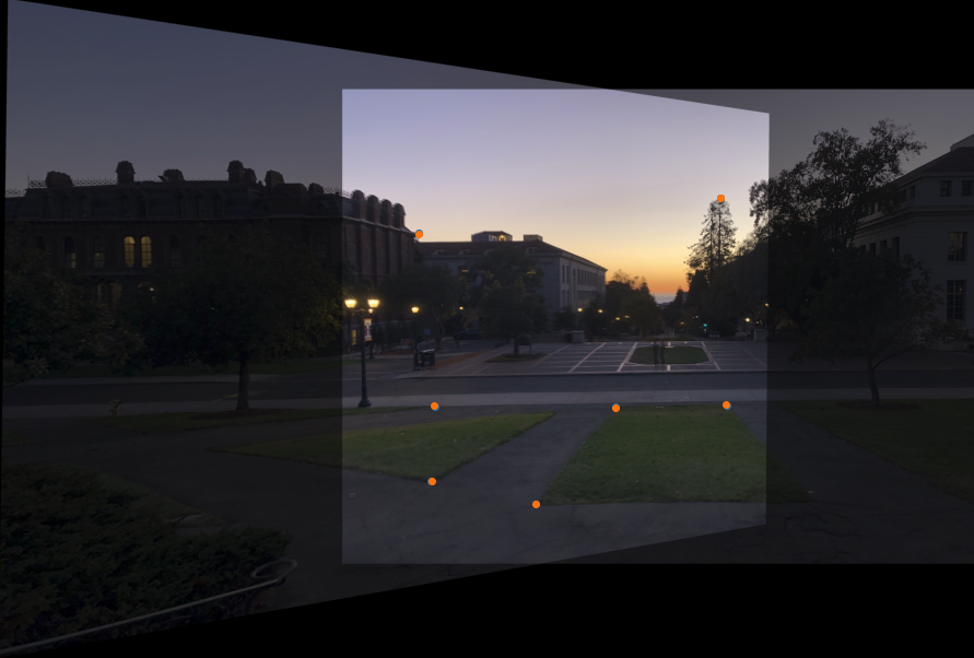 Half-Merged Campanile Way Dusk w/ Points
|
Image Rectification
With the warping function completed, I could now rectify images. More specifically, I could take images that have planar surfaces at an angle and center them to be frontal-parallel. To do so, I took example images
and chose four correspondence points that outlined the planar surface I want to be frontal-parallel. Then, I defined mapped points for them by hand that were rectangular (so I essentially made them be corners for an
axis-aligned rectangle). With the warping function, I could now compute the homography matrix that transforms the correspondence points to the corners of the rectangle that I defined, and warp the image using that homography,
which makes the surface frontal-parallel as intended.
In the example below, I cropped the central grass in the Campanile Way Dusk - Center image and tried to rectify the grass to be flat, as if I was looking at it from a bird's-eye view. It was interesting to see the
patches of grass to the left and right in the image were also rectified to match and align with the central grass portion.
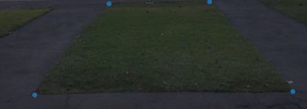 Campanile Way Grass w/ Points
|
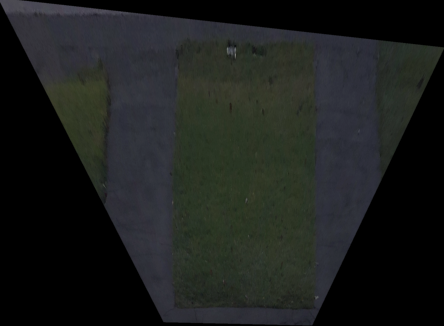 Rectified Campanile Way Grass
|
In this second example, I rectified my dresser that was at an angle in the original picture. It was super interesting to see how the bed that was just in the corner of the image also got perfectly aligned, so it looks
like the rectified image was a picture taken by someone sitting on the bed and looking at the dresser and door.
 Angled Dresser (Original Picture)
|
 Rectified Dresser
|
Blending the Images into a Mosaic
With the warping code creating images large enough to have a warped image a and image b, I blended them together with weighted averaging/alpha blending. To do so, I first computed a mask that represented where the warped image
a and image b overlapped (which is the area that needs to be blended together). I then found the middle point in that mask and created a new image of the same size as what will be the blended image with 1's to the left
of that midpoint and 0's to the right of that midpoint. With this, I applied a gaussian filter with standard deviation 250 to create a smoother transition between left and right. This image with the gaussian filter applied represents
the alpha for the left image (so 1 - the image is the alpha for the right image) post-warp.
This gaussian filter takes an extremely long time to compute because the image has so many pixels. To optimize the speed, since we know the filter/alpha image is the same from top to bottom but varies from left to right, as you can see
in the image of the alpha image below. As a result, since the standard deviation doesn't change, I took a single row of this image to memoize, and for any other image warps I rotate the pixels from left to right (or right to left)
until the center of the blending is the midpoint of the mask for the new image. Then, I stack this row repeatedly on top of itself and right-pad with 0's until the image shape matches that of the images I am blending
together. This saves the time of recomputing the gaussian from scratch over and over, heavily speeding up my code. An example of the alpha image generated with 1000 rows and 5000 columns is below:
 Gaussian Alpha Image Applied to the Left Warped Image for Blending
|
Finally, to blend, I simply multiply the left warped image by the alpha image and add that to the right warped image multiplied by 1 minus the alpha image, producing the results below:
|
Campanile Way Dusk - Left
|
|
Campanile Way Dusk - Center
|
|
 Campanile Way Dusk Merged
|
|
Campanile Way Day - Left
|
|
Campanile Way Dusk - Center
|
|
 Campanile Way Day Merged
|
|
Hearst Mining Circle - Left
|
|
Hearst Mining Circle - Right
|
|
 Hearst Mining Circle Merged
|
In the Hearst Mining Circle Merged Image above, we can see that the entire image is crisp. This was actually my second try merging these images together. In the image below, you can see the first attempt.
If you zoom in you can see some interesting blurring on the middle door, which is in the center of the overlapping area of the two original images.
I believe this blur can be attributed to the selection of correspondence points not perfectly overlapping, causing some differences in pixel values between the left and right warped images,
essentially causing a convolution of those pixels resulting in the blur. After retrying selecting correspondence points, I got the merged image above, which does not have that blurring.
 Merged Hearst Mining Circle with Blurry Overlap
|
After merging the dusk images for Campanile Way, I wanted to try merging more images, more specifically an image angled further right that I took, in order to test the ability of my implementation to merge
any number of images together. The result is shown below!
|
Campanile Way Dusk - Left and Center Merged
|
 Campanile Way Dusk - Right
|
|
 Full Campanile Way Dusk Merged
|
Lessons Learned
I learned a lot about warping images that have non-affine transformations between them. It was super surprising and interesting to see the sheer accuracy of these techniques at finding the transformation
between the images, all from selecting some correspondence points. I also learned about the importance of using different blending techniques. I initially tried a linear blend but found that it created weird
coloring issues where it was clear where the bounds of the original images were. As soon as I switched to the Gaussian, I saw those boundaries disappear, resulting in the cleaner images above. I also thought the
rectification was interesting. The results, especially with the dresser image and how it captured the bed in the corner as I described above, were fascinating and I hope to explore them more in the future.