Project 4a: Image Warping and Mosaicing
Simona Aksman
Contents
Part 1: Shoot the Pictures
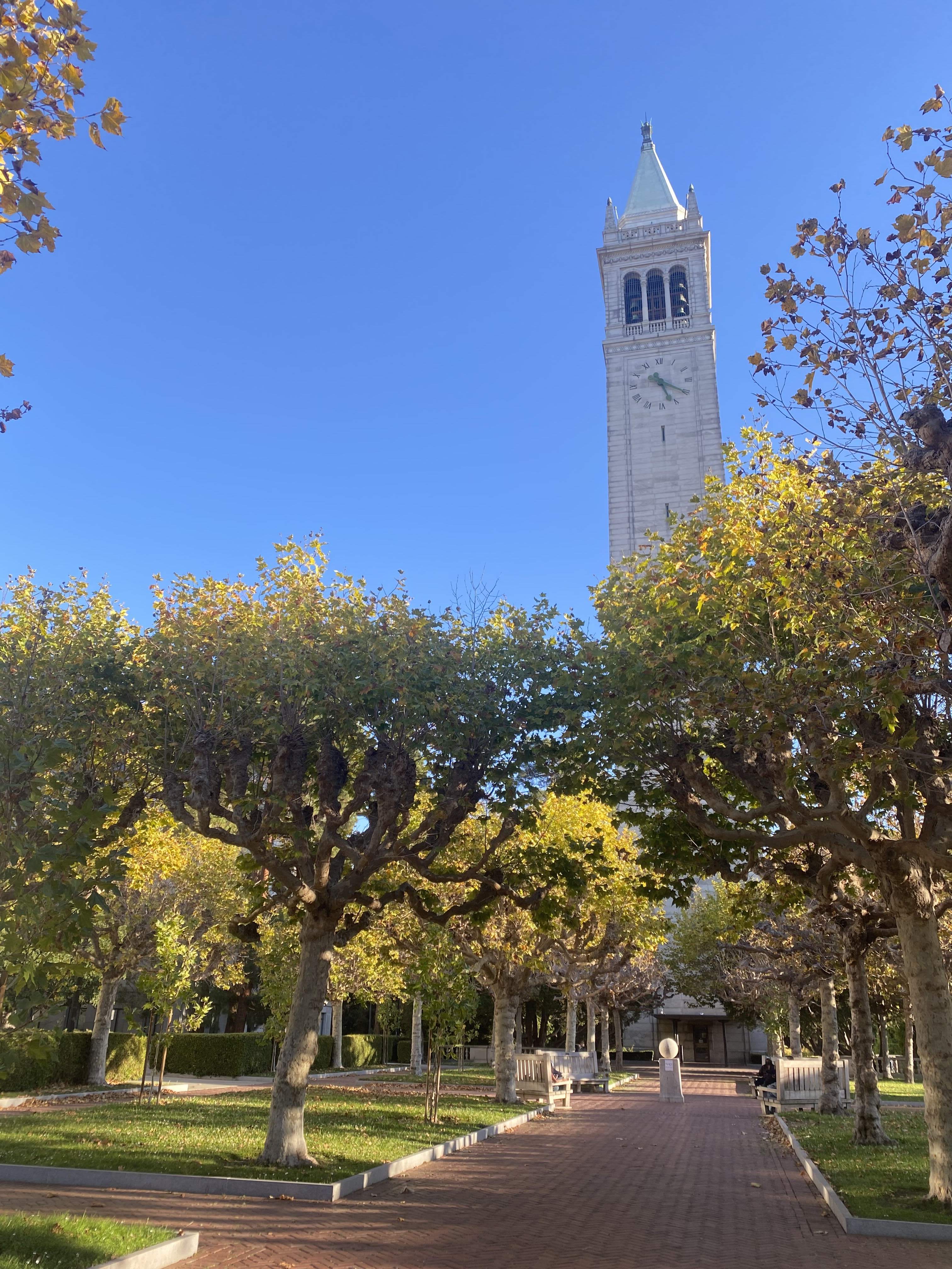
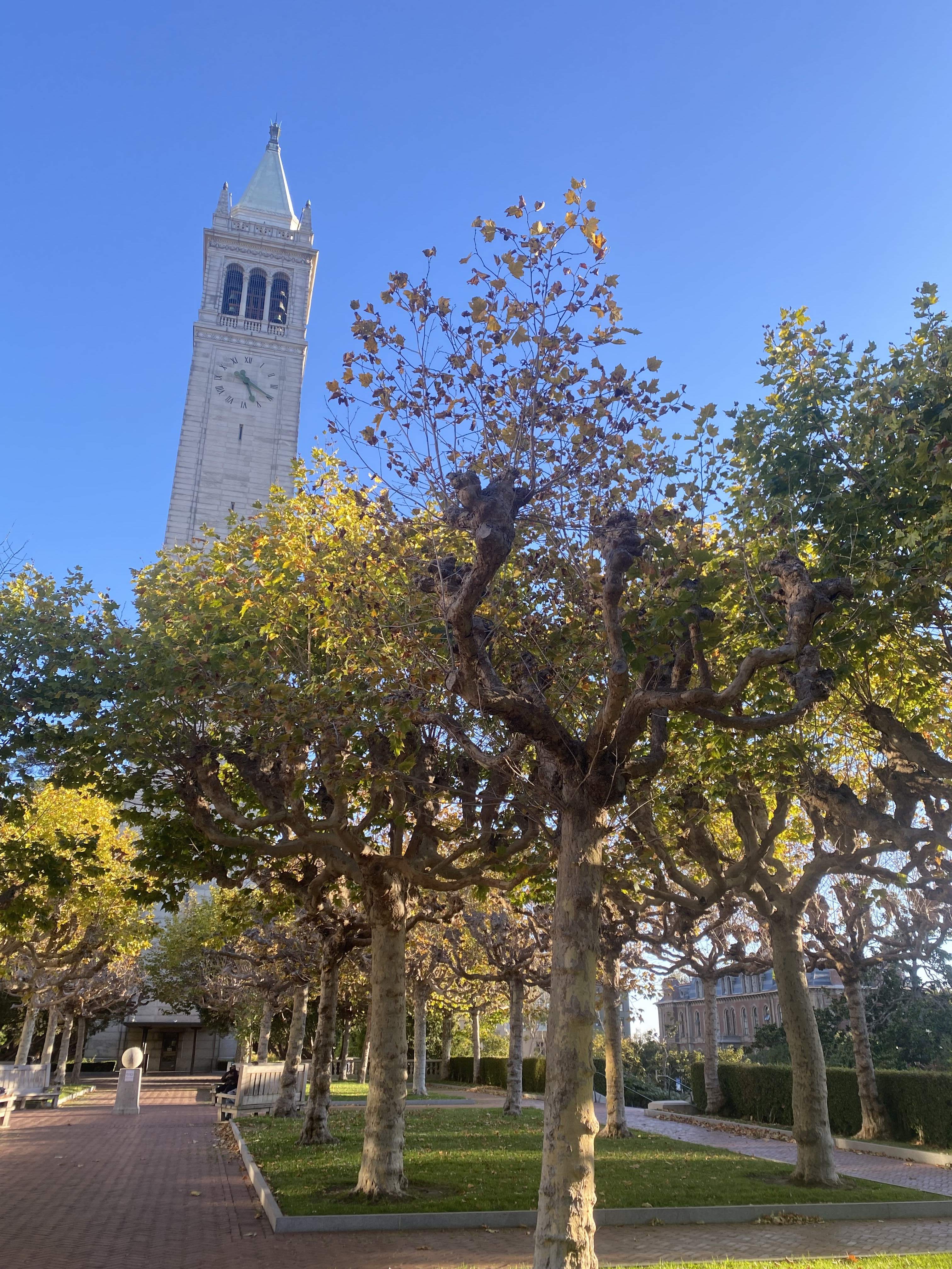
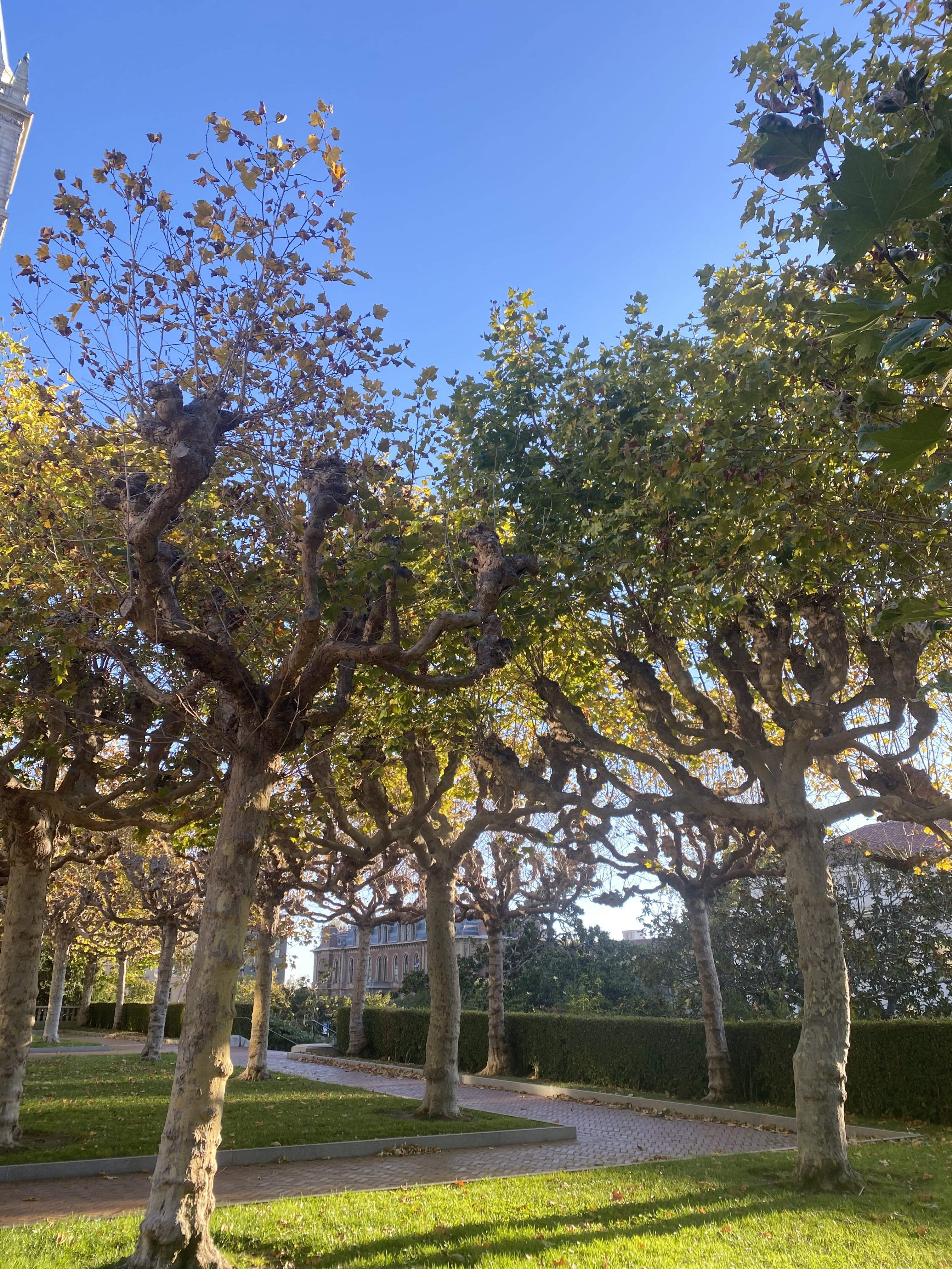
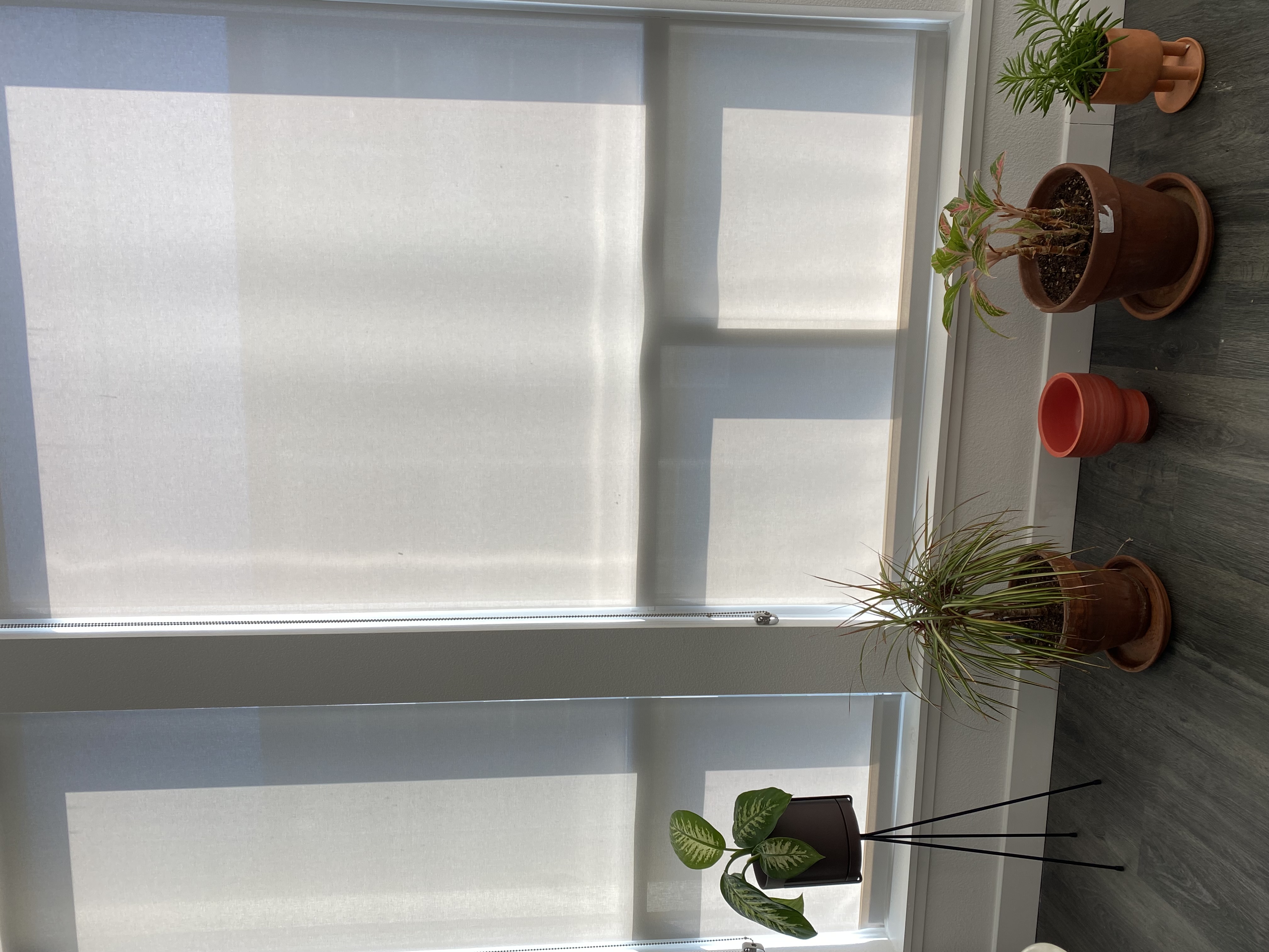
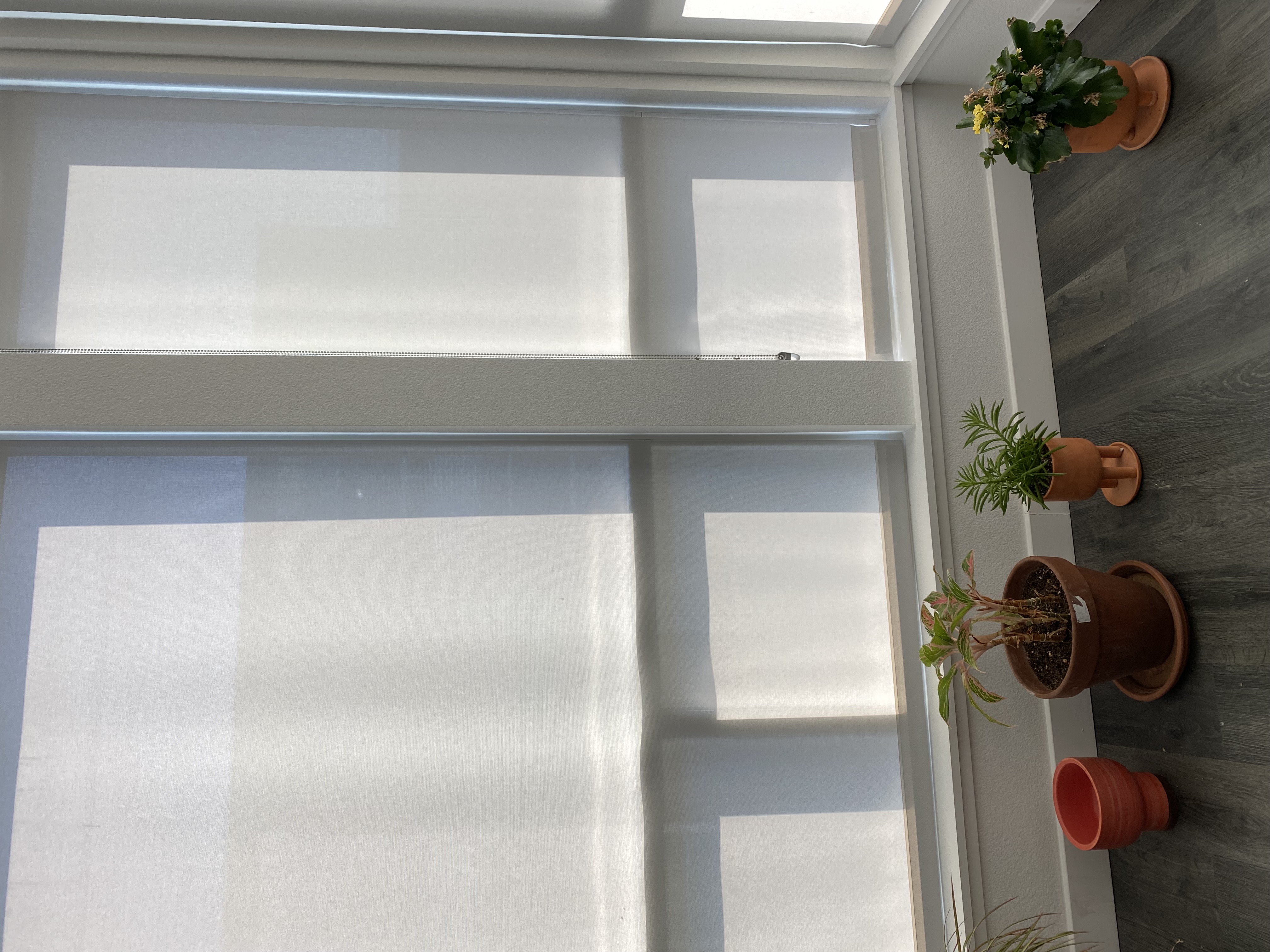
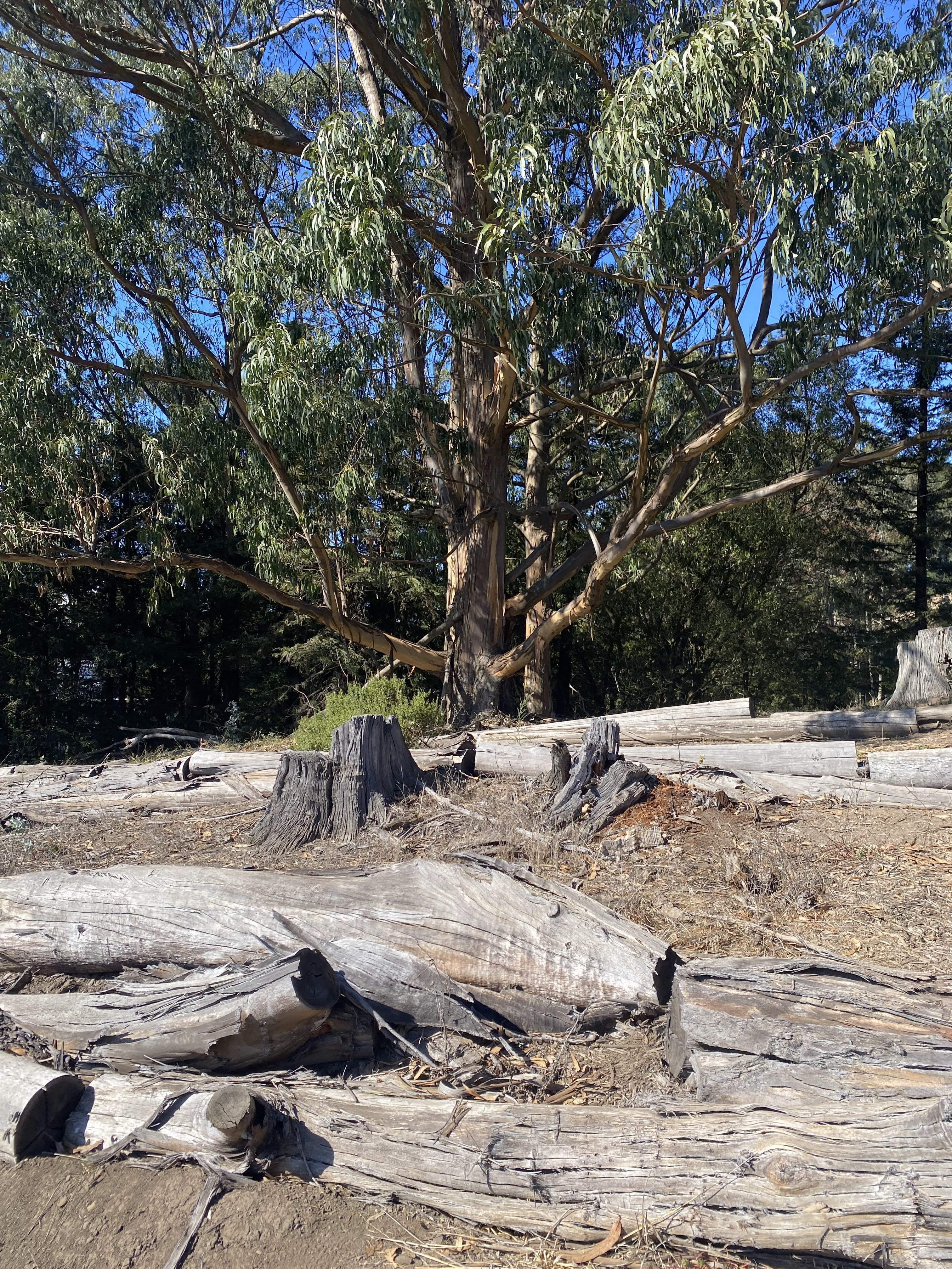
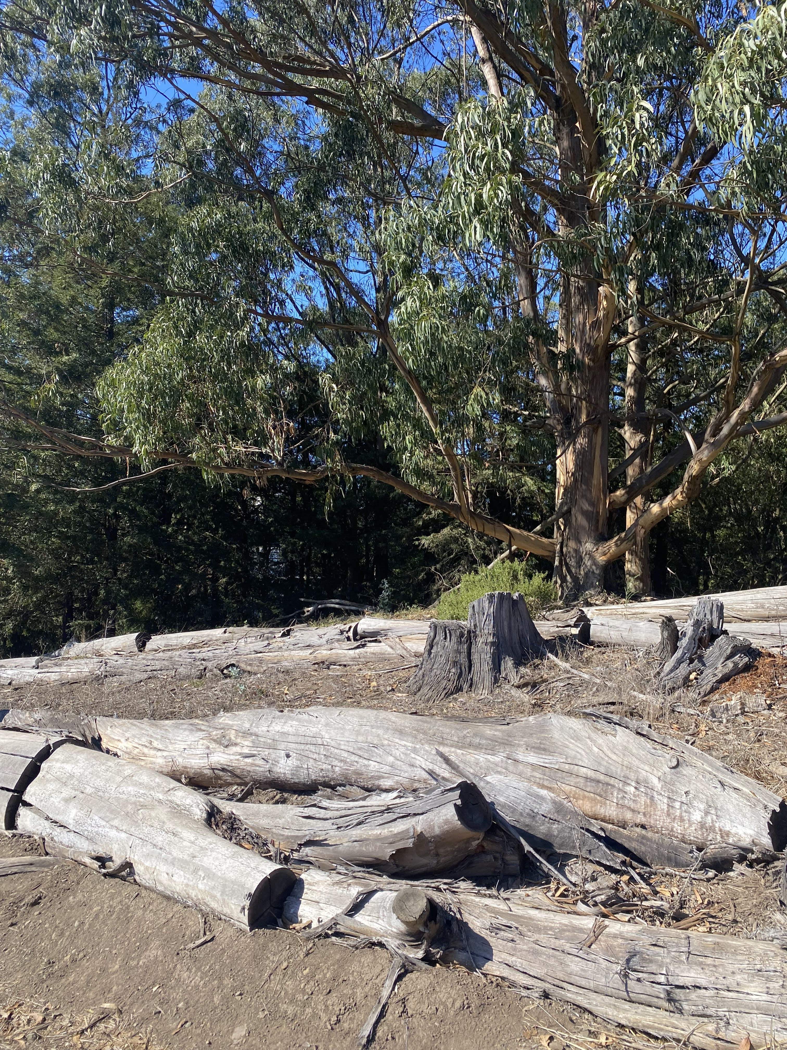
To start, I shot some indoor and outdoor photos using the approach outlined in the assignment prompt. See below for the images I selected for the project.
Part 2: Recover Homographies
Next I worked on setting up a function that recovers a homography given at least four correspondences. At least four are needed because they produce the 8 degrees of freedom that allow you to compute a homography. However, since 4 correspondences do not always produce an accurate homography, we use an approach that supports more than 4 correspondences: least squares. To set up my correspondence to run least squares, I first expanded the homography equation outlined in class:
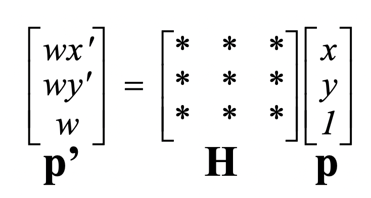
into the equation of this form:
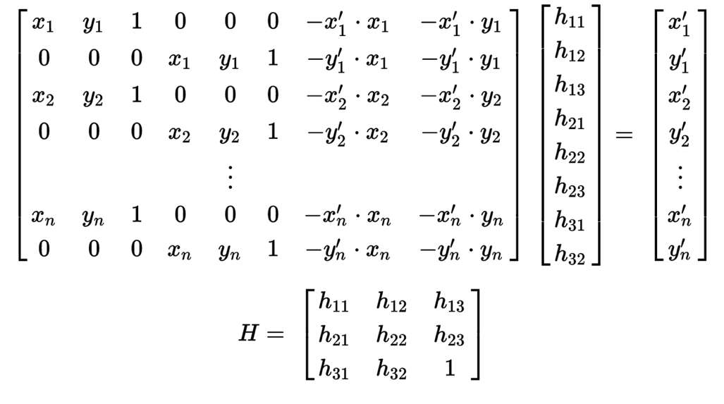
and then solved it via a least squares solver (which does this):

where A is is the 2n x 8 coefficient matrix, b is the 2n x 1 dependent value matrix, and x is the least-squares solution which minimizes the Euclidean distance between b and Ax.
Part 3: Warp the Images
Then I wrote the warping function warpImage, which takes as input the image and the homography, applies inverse warping to transform the shape of the image, and then fills in the colors of the image and background using an interpolation function. The warpImage function is similar to the affine warp function I wrote for project 3, except it also handles empty pixel values, which homography transforms can generate and affine transforms do not.
Part 4: Image Rectification
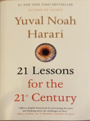
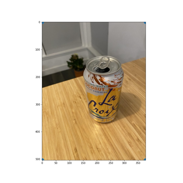
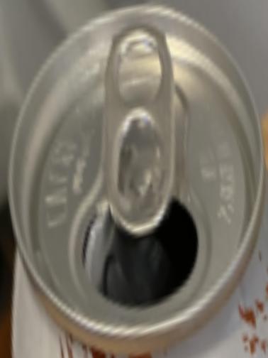
Once I wrote the warping function, I was ready to test it out. To do so, I "rectified" images: I took images which contained objects with planar surfaces and applied a homography tranformation to get an image of the frontal-parallel view of the surface. This seemed to work well overall, though some details appear blurry i.e. the small text on the book in my first example. In addition, some details were not planar in the image so they cannot be recovered i.e. the inner ridges of the LaCroix can.
Image with source mapping
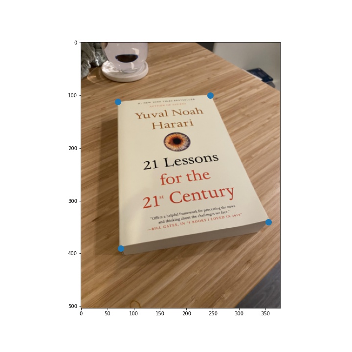
Image with destination mapping

Rectified image

Part 5: Blend the images into a mosaic
Finally, I blended the images I shot in part 1. Setting up the correspondences to ensure correct image alignment was pretty tricky, and I ended up having to do them several times to get them right. For each pair of images that I blended, I set up 10 to 20 correspondences of key features in the image depending on the image. I found that it was helped to label keypoints in a wide range of the image. When I focused my labeling efforts on just one section of an image, sometimes the other parts of the image wouldn't be well aligned.
As for how I did the blending, I found that I had decent results when I took the minimum of all of the pixel values in the images I was mosaicing (or the maximum when there's a black background). Unfortunately, there are still some traces of edge artifacts in the images after applying this blending approach. I experimented with several blending approaches (2-band Laplacian stack, alpha blending) but had trouble getting those to work well. If I have time next week, I will continue to experiment with ways to reduce the edge artifacts. In particular, I would like to try out gradient blending.
Original images
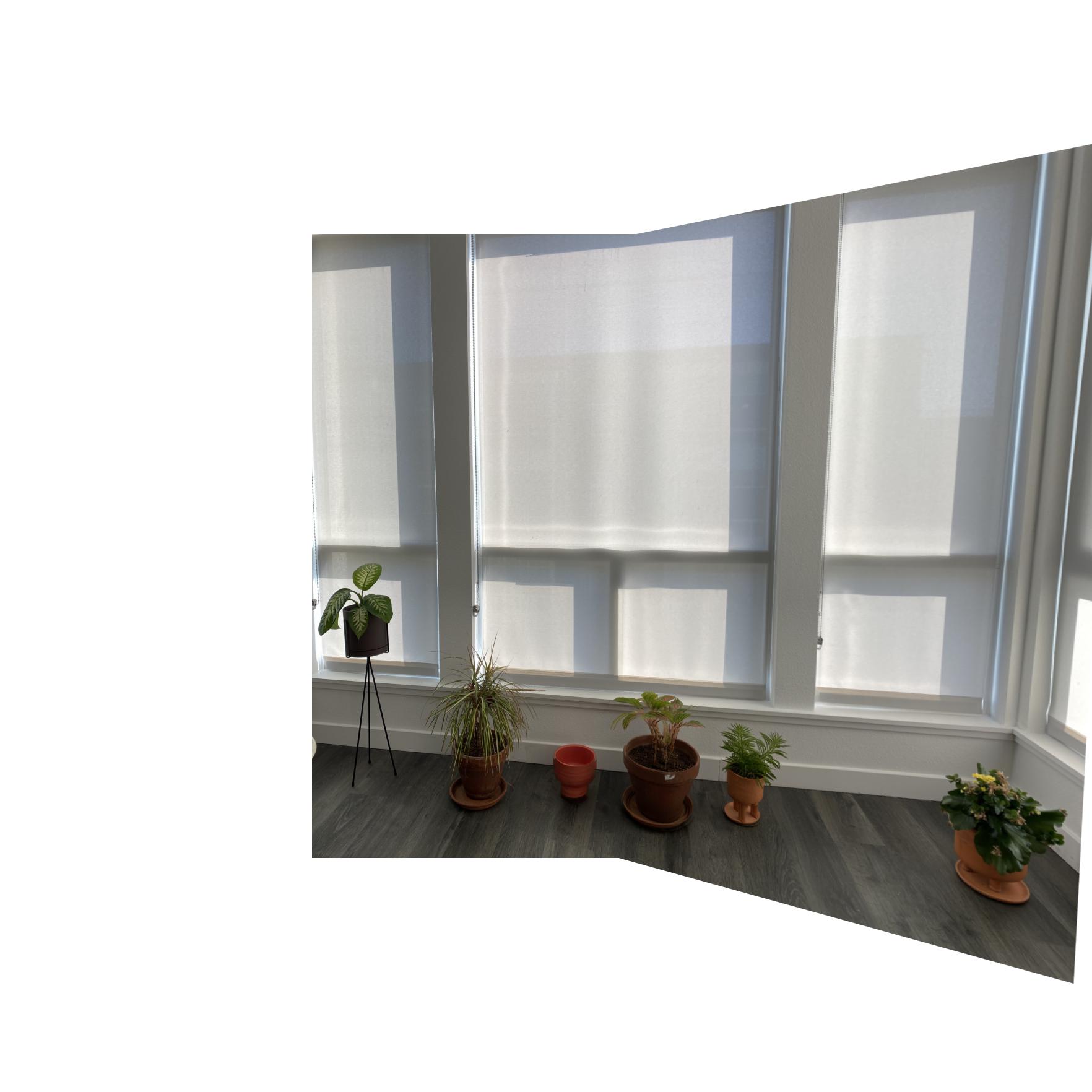
Mosaic
Original images
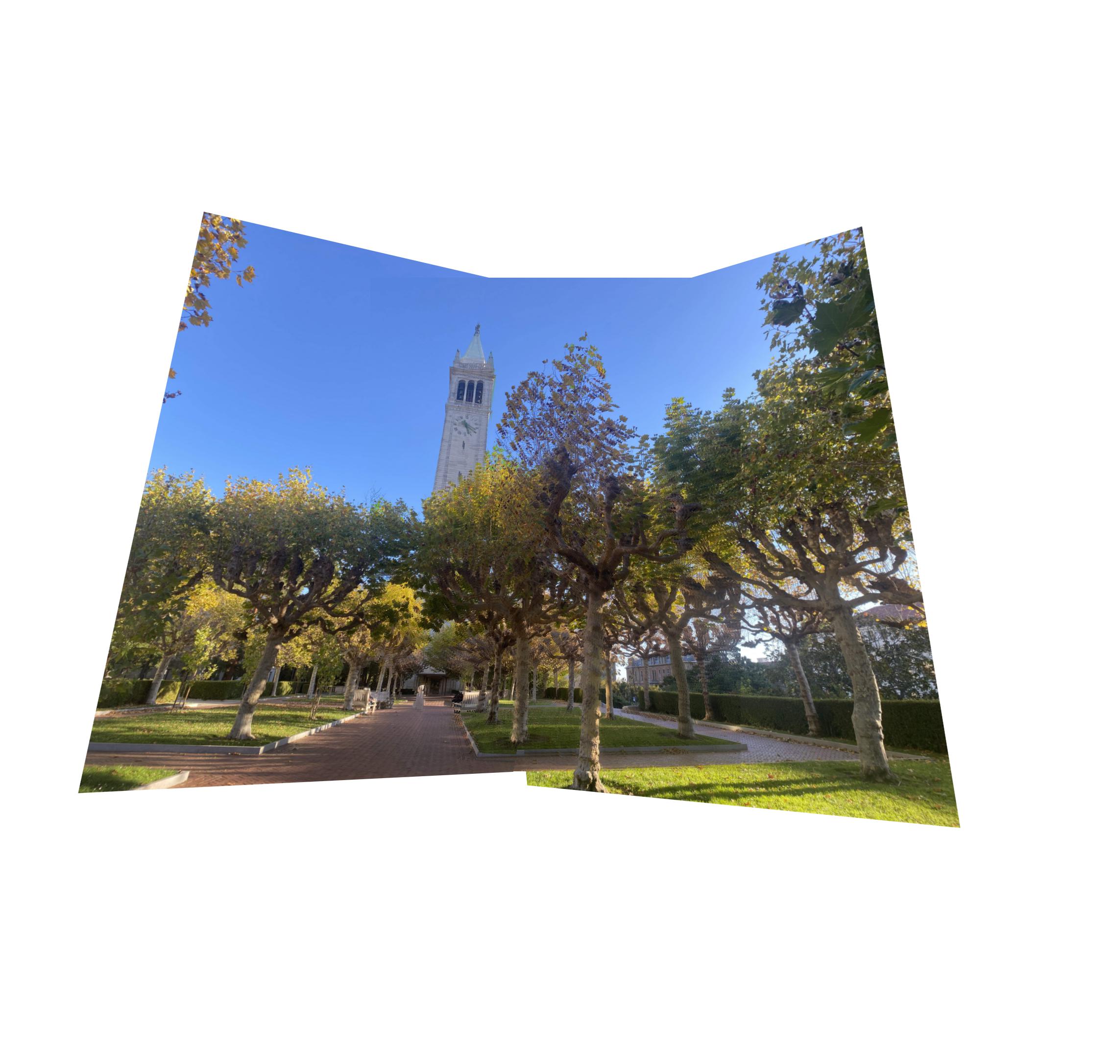
Mosaic
Original images
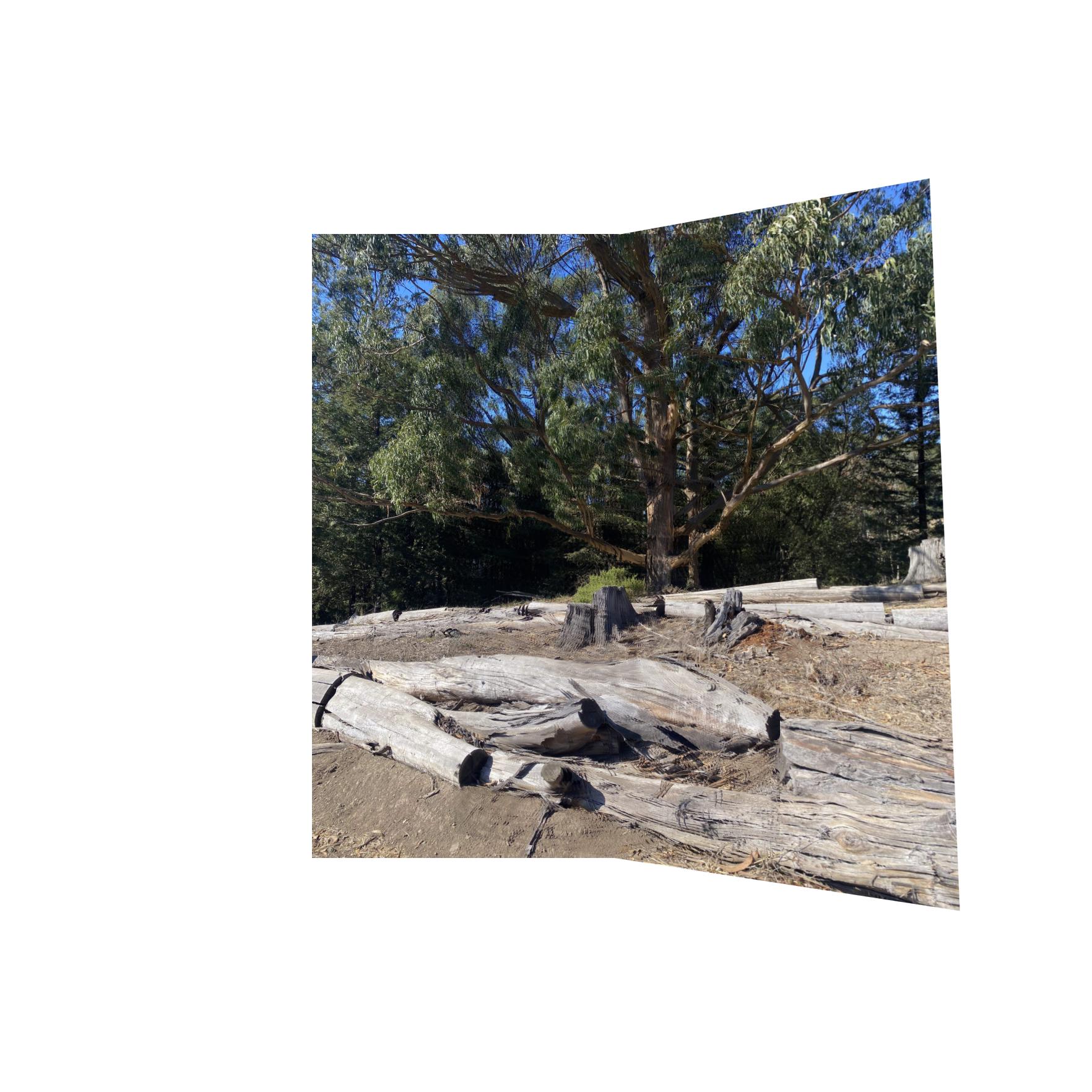
Mosaic
Reflections
This project was really cool because it gave me a visual intuition for how least squares estimation works. It was interesting to watch how my alignments got better as I got better at identifying keypoint candidates and piped in more of them. However, it was also quite time consuming and challenging to label the keypoints well (especially when trees were involved). I am excited for the next part of the project where we start to use methods that automate keypoint detection.