Jeremy Warner — jeremy.warner at berkeley.edu
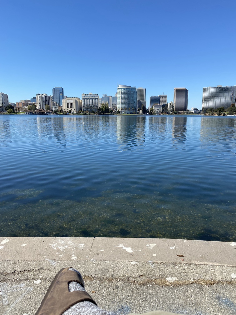
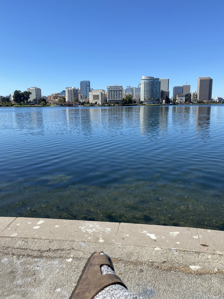
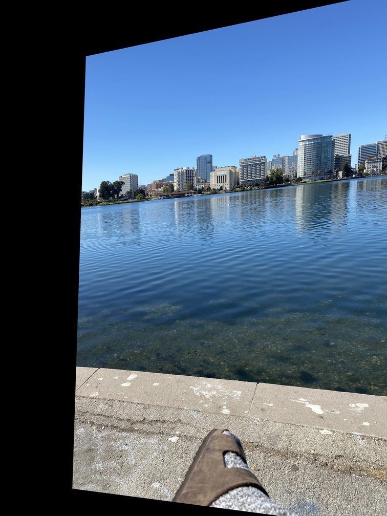
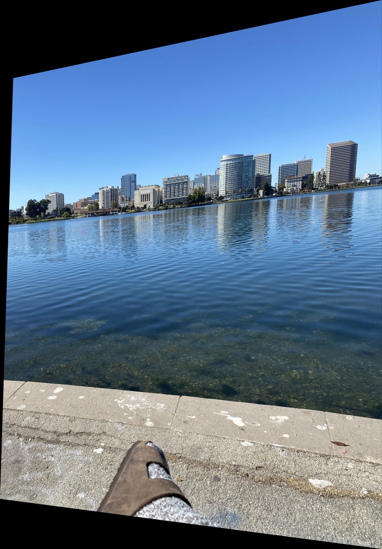
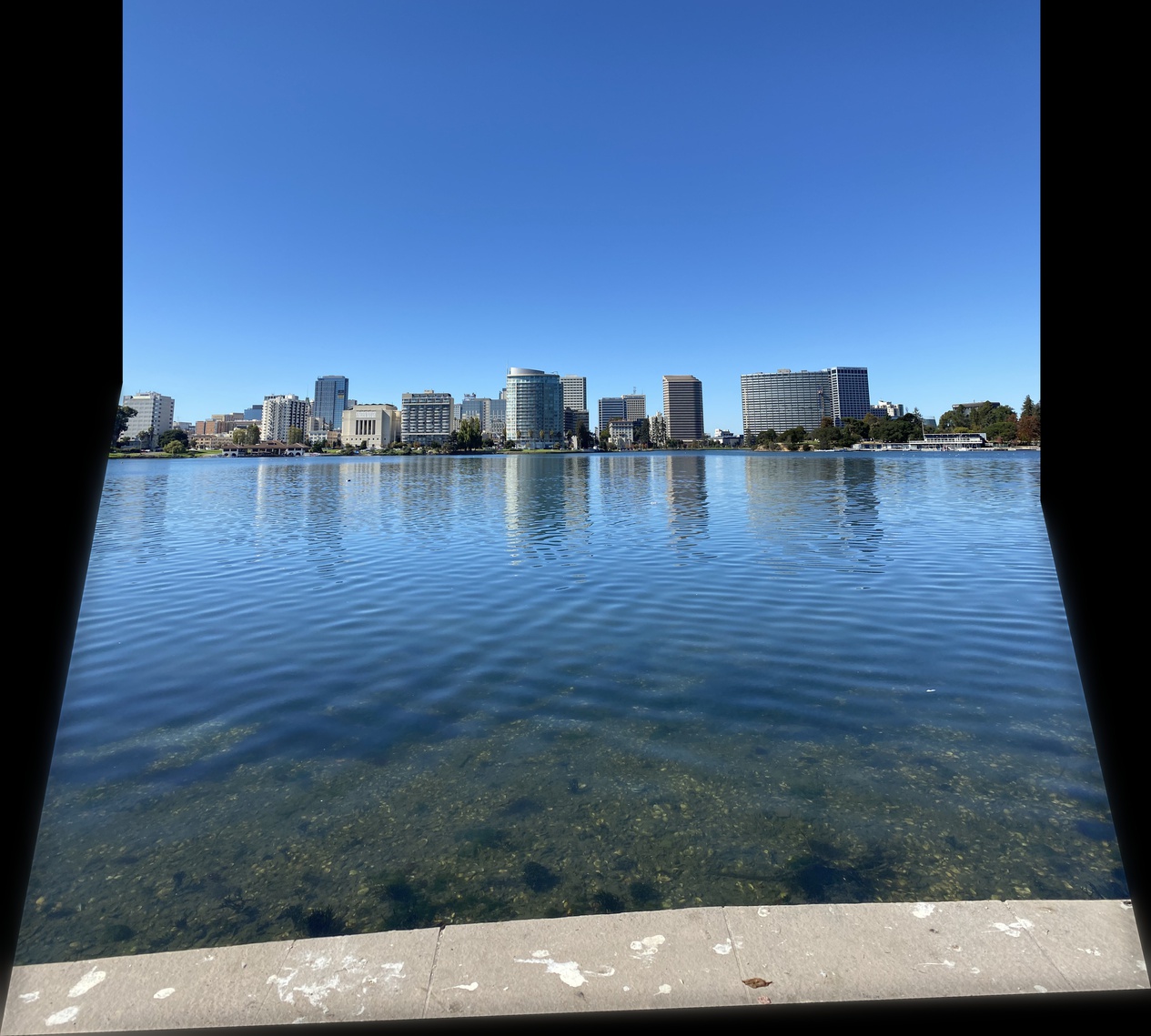
I shot three good scenes for merging images: lake (tiled vertically), desk, and room.
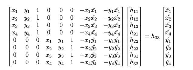
Implementing H = computeH(im1_pts,im2_pts):
im2_pts flattened as the b vector (Nx1).np.linalg.lstsq (Least Squares) to compute x, from min(|Ax−b|).An example with four pairs of points:
Ours: computeH(lake1_pts, lake2_pts)
[[ 7.01676933e-01 -3.11523405e-02  6.71168430e+02]
[-1.93303430e-01  8.04904281e-01  4.39912882e+02]
[-7.62728811e-05 -8.62315758e-06  1.00000000e+00]]
cv2: cv2.findHomography(lake1_pts, lake2_pts)
[[ 7.01679953e-01 -3.11513492e-02  6.71164879e+02]
[-1.93302319e-01  8.04908423e-01  4.39904713e+02]
[-7.62725971e-05 -8.62262262e-06  1.00000000e+00]]
Selecting points is very tricky. For Part A, I was careful to define good points (often zooming w/ ginput per point), but implementing the automatic tuning of correspondences would be a great augmentation I will include for Part B.
Computing warpImage(im, H): Apply the transformation H to each pixel in im and interpolate these pixel colors with cv2.remap, by default generating an output image mirroring the input’s size.

Similar to cv2.warpPerspective, my warpImage accepts an optional size parameter which determines the output size of the projected image. This enables me to also create a warpImageFull function that retains the entire projected image in the final canvas by computing the bounds of the projected input image and passing that in as size, along with a new translated homography (T * H).
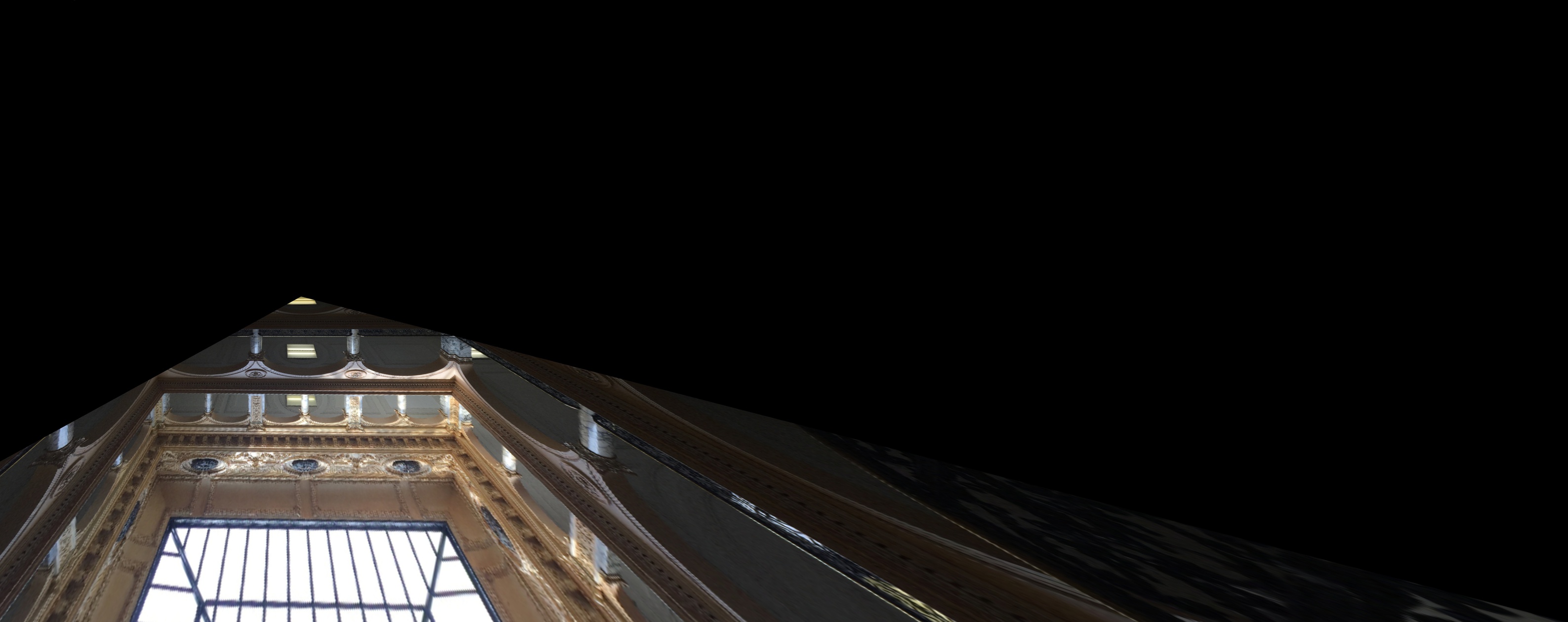
Computing rectify(im , corners): using a square’s corners for one set of points in computeH allows us to compute and apply a homography to a specific rectangular section of an image.

These images can also be shown “fully” in a manner similar to warpImageFull, where the specified plane is rectified though the rest of the image is also included in the final canvas.

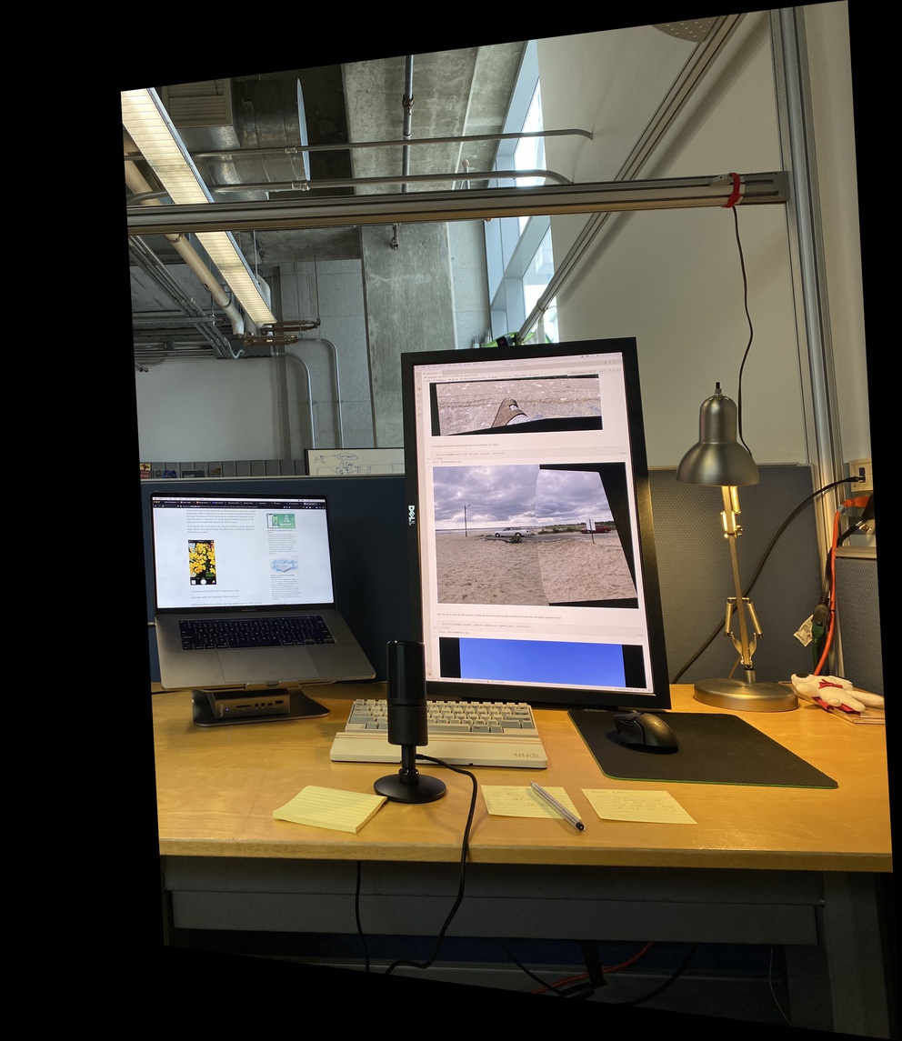
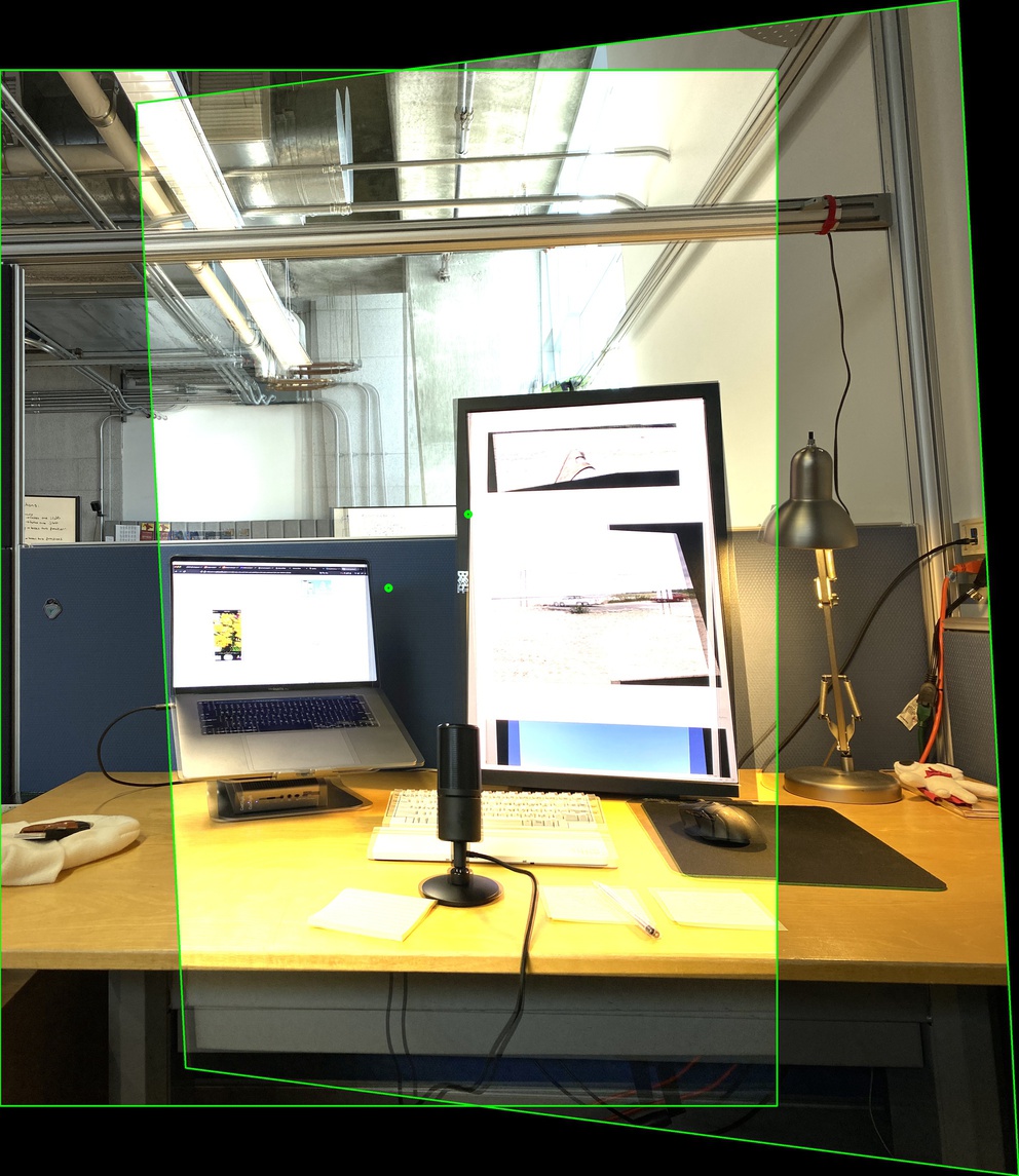
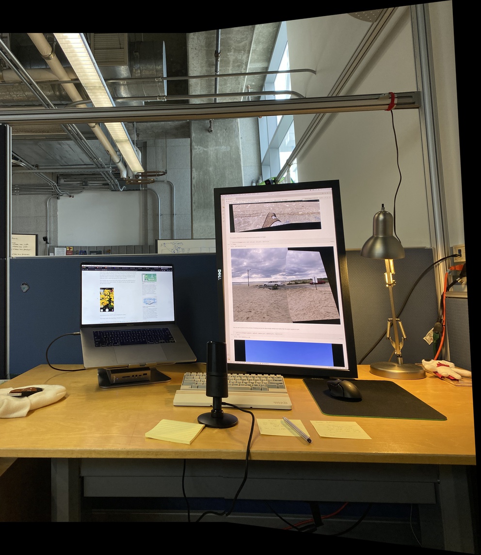
We’ll walk through creating an image mosaic with this desk example.
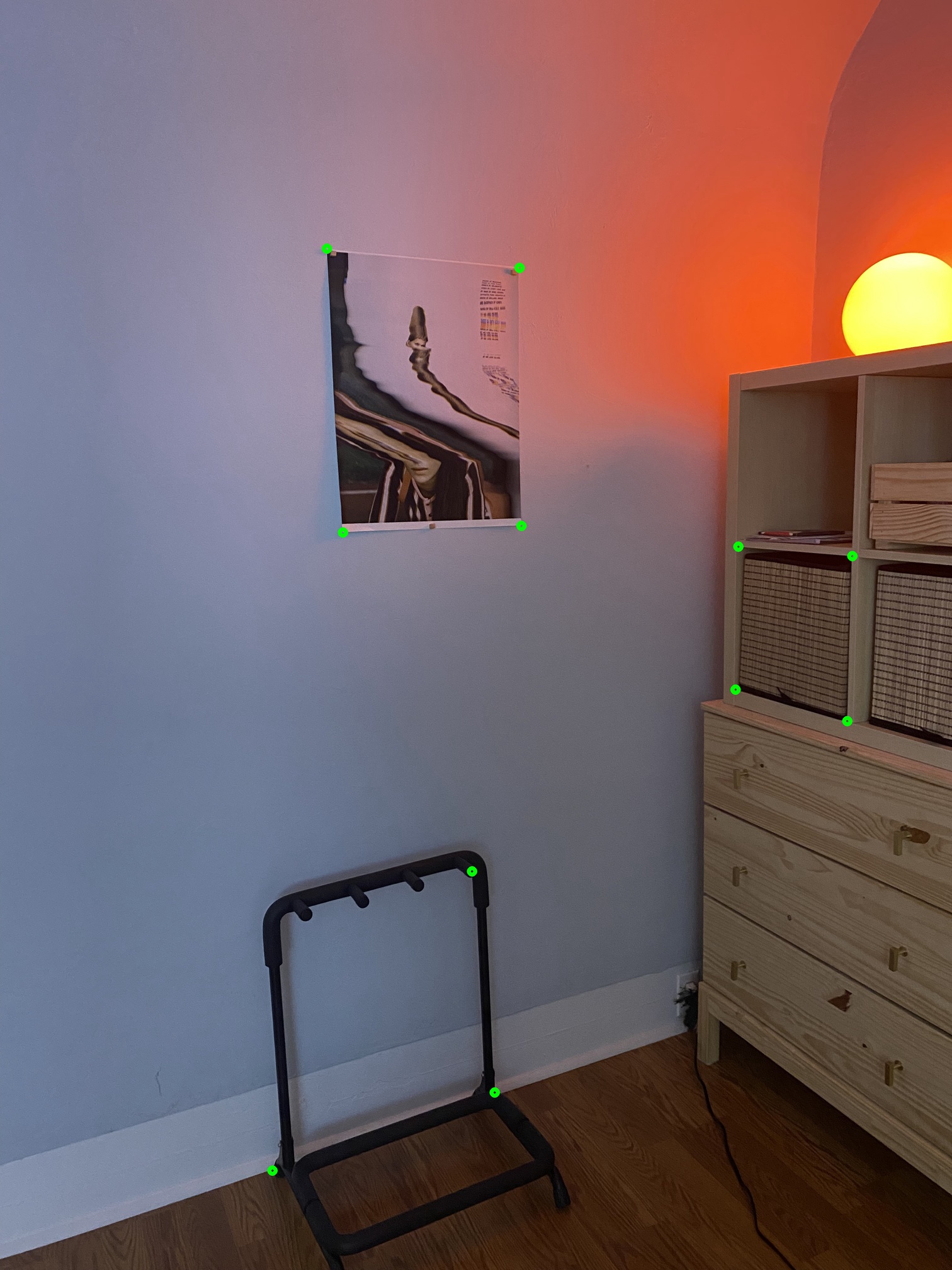
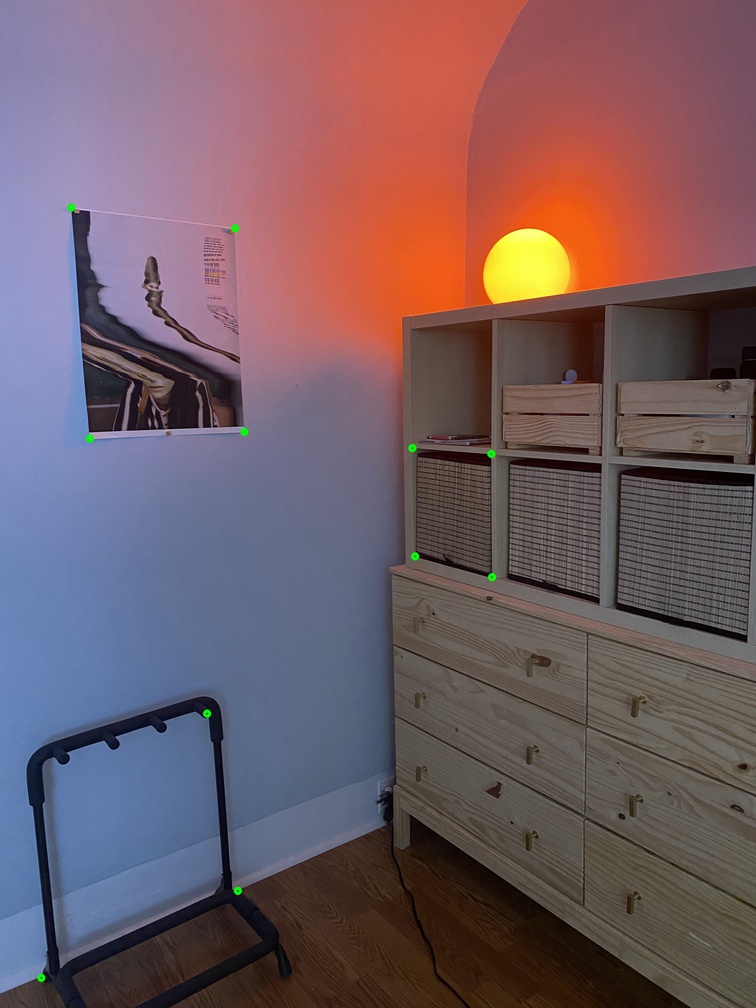
The green points correspond to the manually set point correspondences (N = 6).
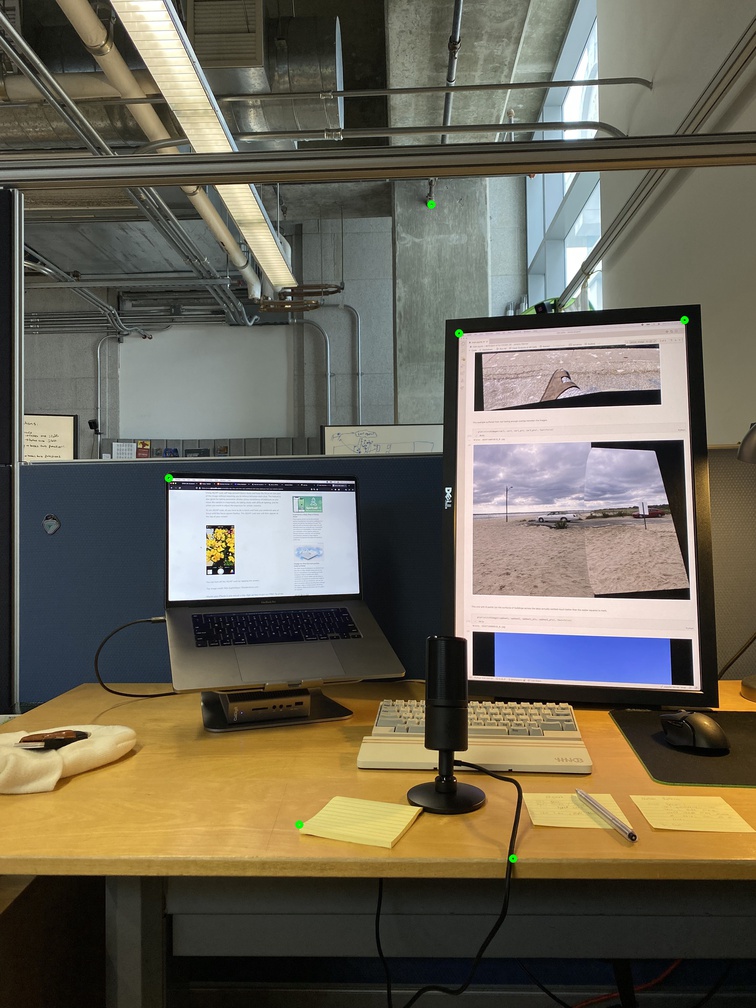
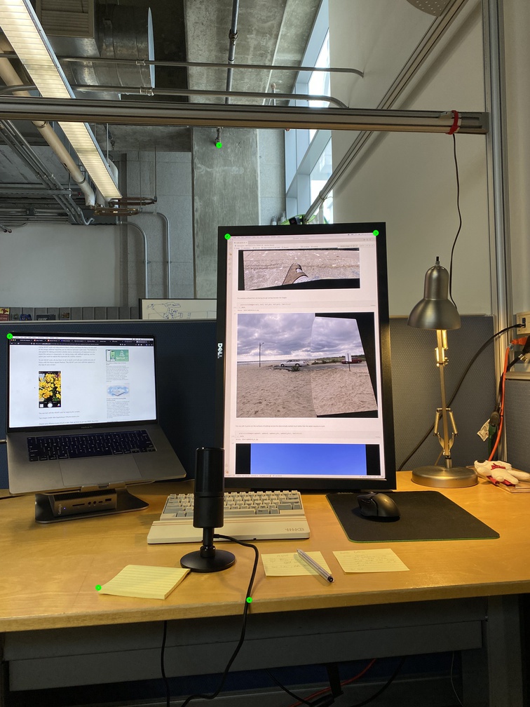
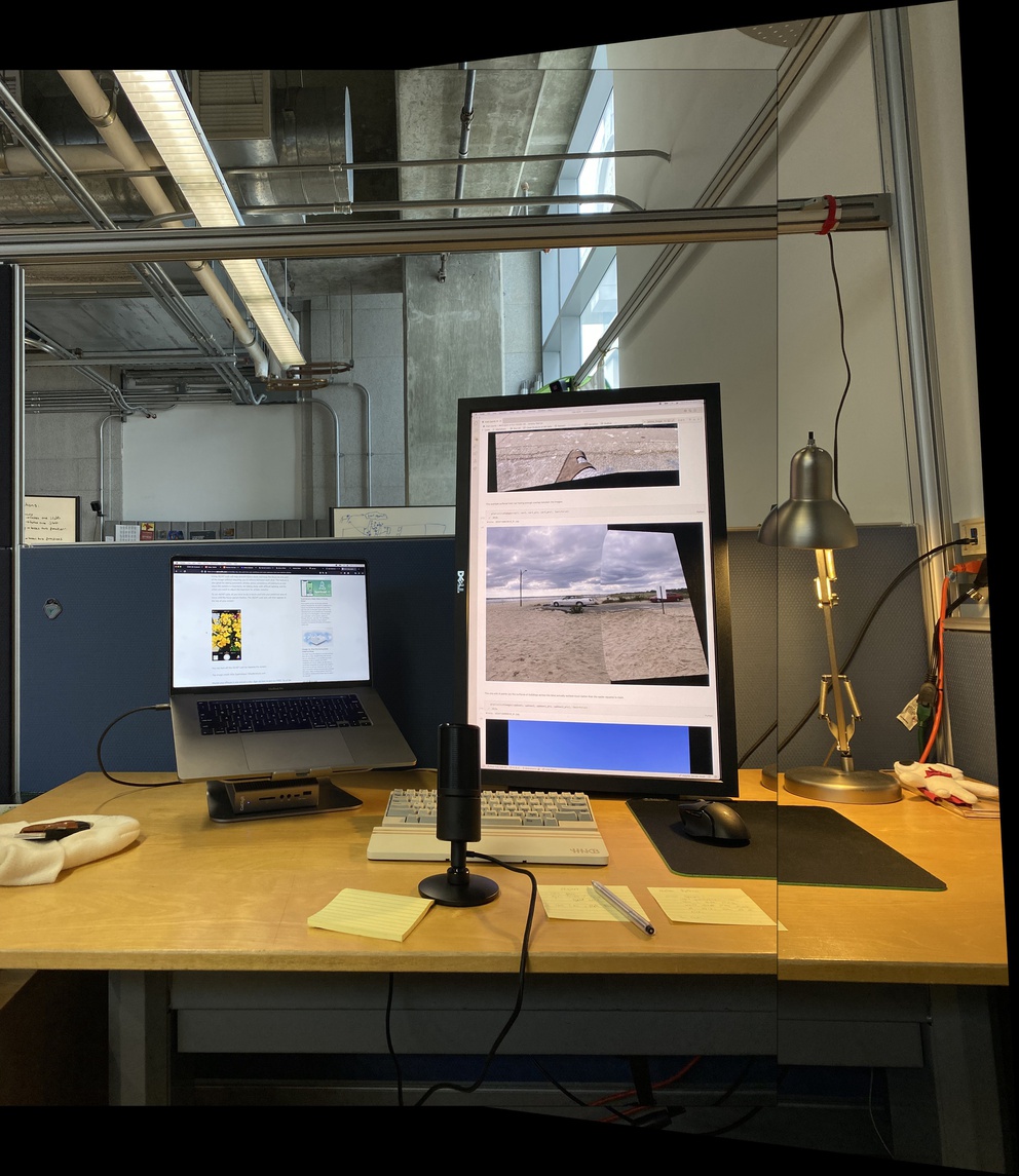
We can compute the homography and overlay the images by simple addition.
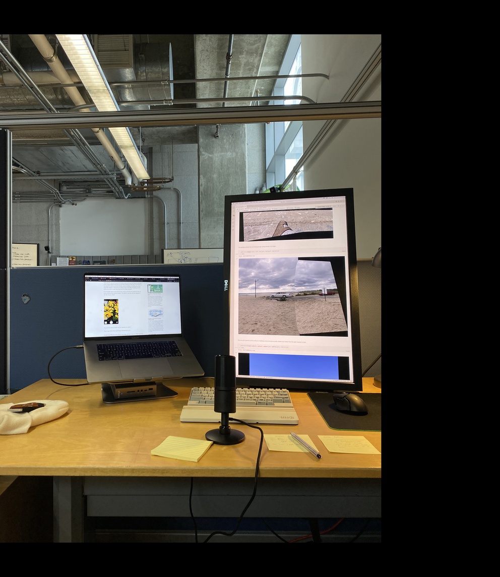
That obviously doesn’t look great, though the images are aligned. We need to compute a mask that allows us to combine the two images nicely. We’ll borrow and update our project 2 image blending code for multi-band blending, but we still need a mask.
One basic mask involves thresholding both images, then masking with the union(L, R) - L, which yields this mask and blended result:
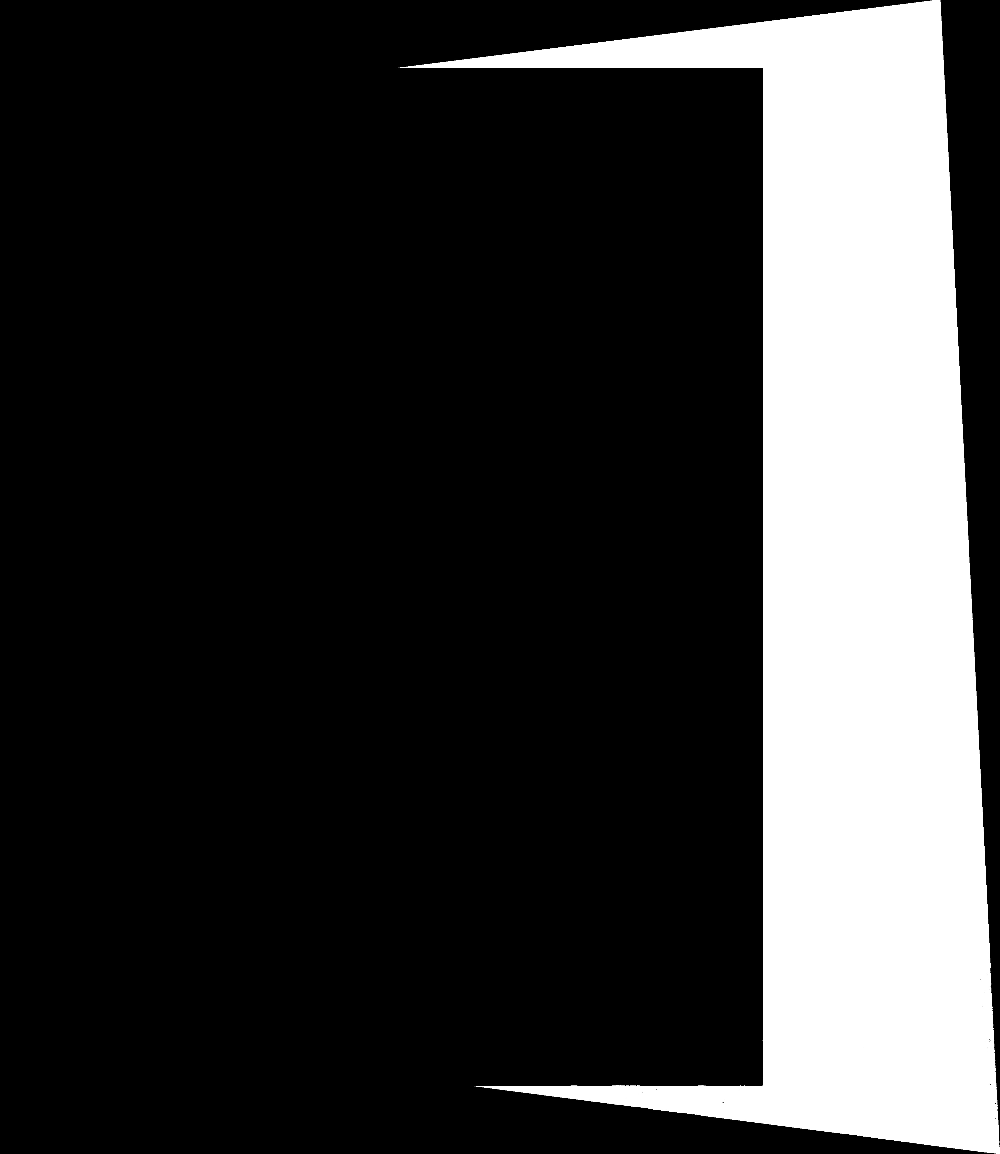
Ok, simple enough but this actually will leave a seam at cases like this where the edge of one region is black. Unlike our project 2 example where the images were defined on both sides of the mask, the black background from the left image is being blended into the seam, creating a clear marker. This is also generally true for every edge of the images that aren’t aligned with the canvas edge, though it is most noticeable at the seam.
Let’s simplify the mask into the overlapping static image from the warped image. We’ll compute two intersection points of the projected bounding boxes, and fill the mask region.
Nice! The seam is now hidden in the image.
The strategy for finding the right points to polyfilly is to get each of the lines of the bounding boxes, defined by two corner points that lie on them. With these lines, we compute where they intersect with the lines of the other bounding boxes, generating 16 intersection points (barring any parallel lines, 4x4). We then take the two with the min joint distance from both bounding boxs. These two intersection points are joined with vertices on the right box that are outside of the left box and drawn with cv2.fillPoly.
Worth noting this doesn’t handle cases where the boxes don’t intersect or are entirely within. In those cases, we won’t have the black aliasing effect on that inner seam since image data is defined on both sides of the region mask, so the case isn’t relevant there.
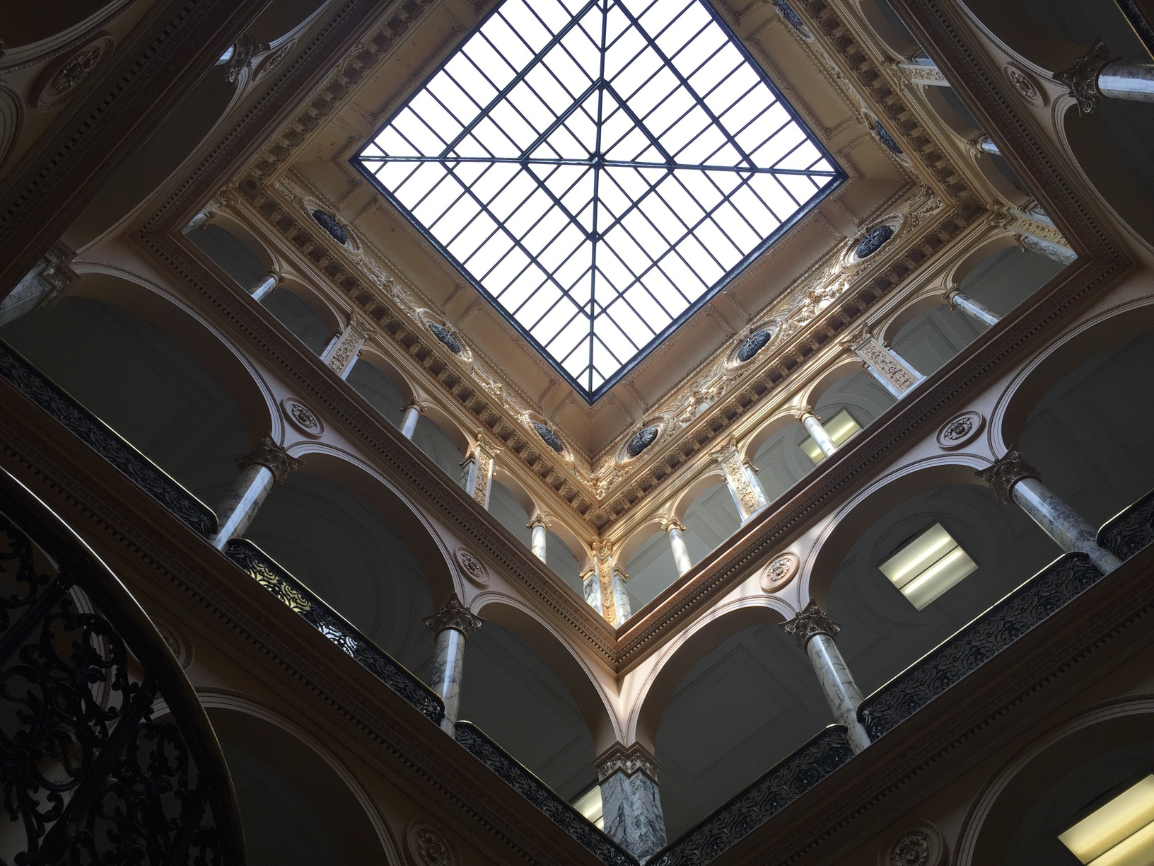
For the room shots, I captured both standard and ultra-wide shots on the iPhone 11 Pro to see the difference in perspective, and to see whether the homography would perform differently due to warping around the ends of the images. Suprisingly, both of them came out well, though you can see some tearing around the outlet towards the bottom left corner of the dresser that is absent in the standard shot.


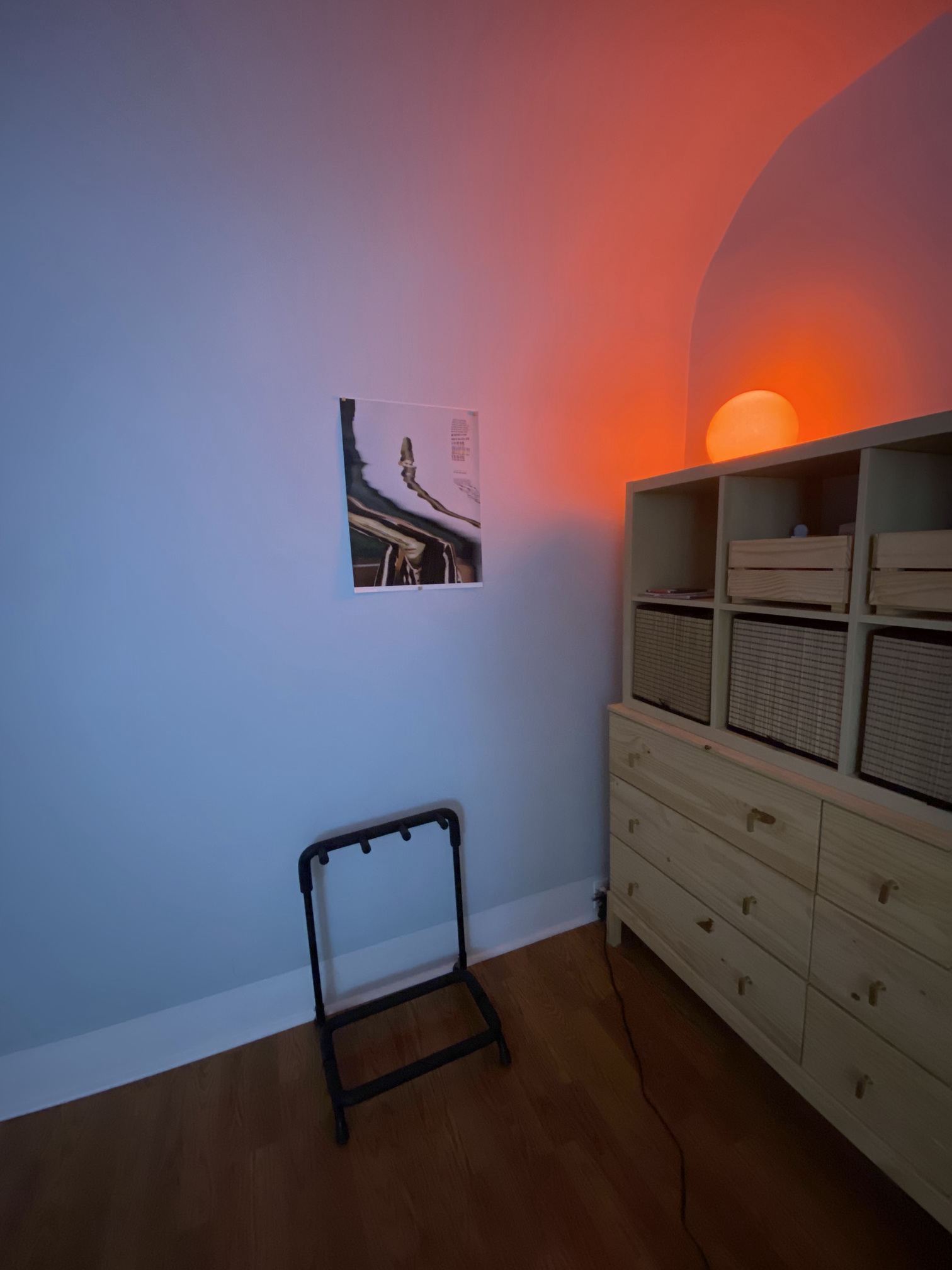
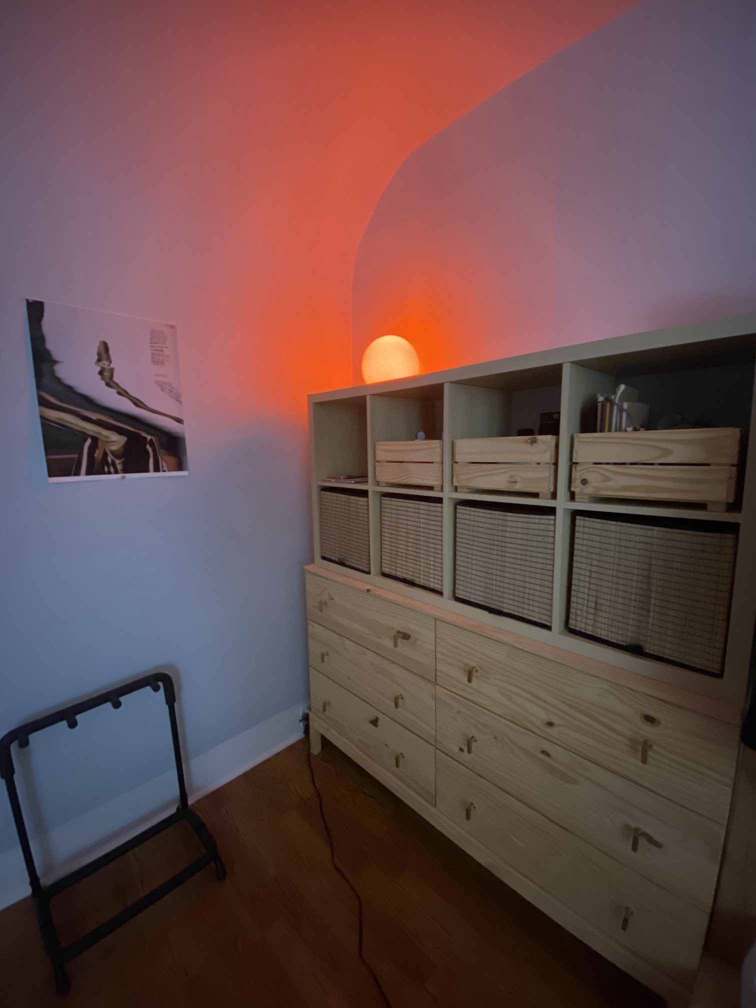
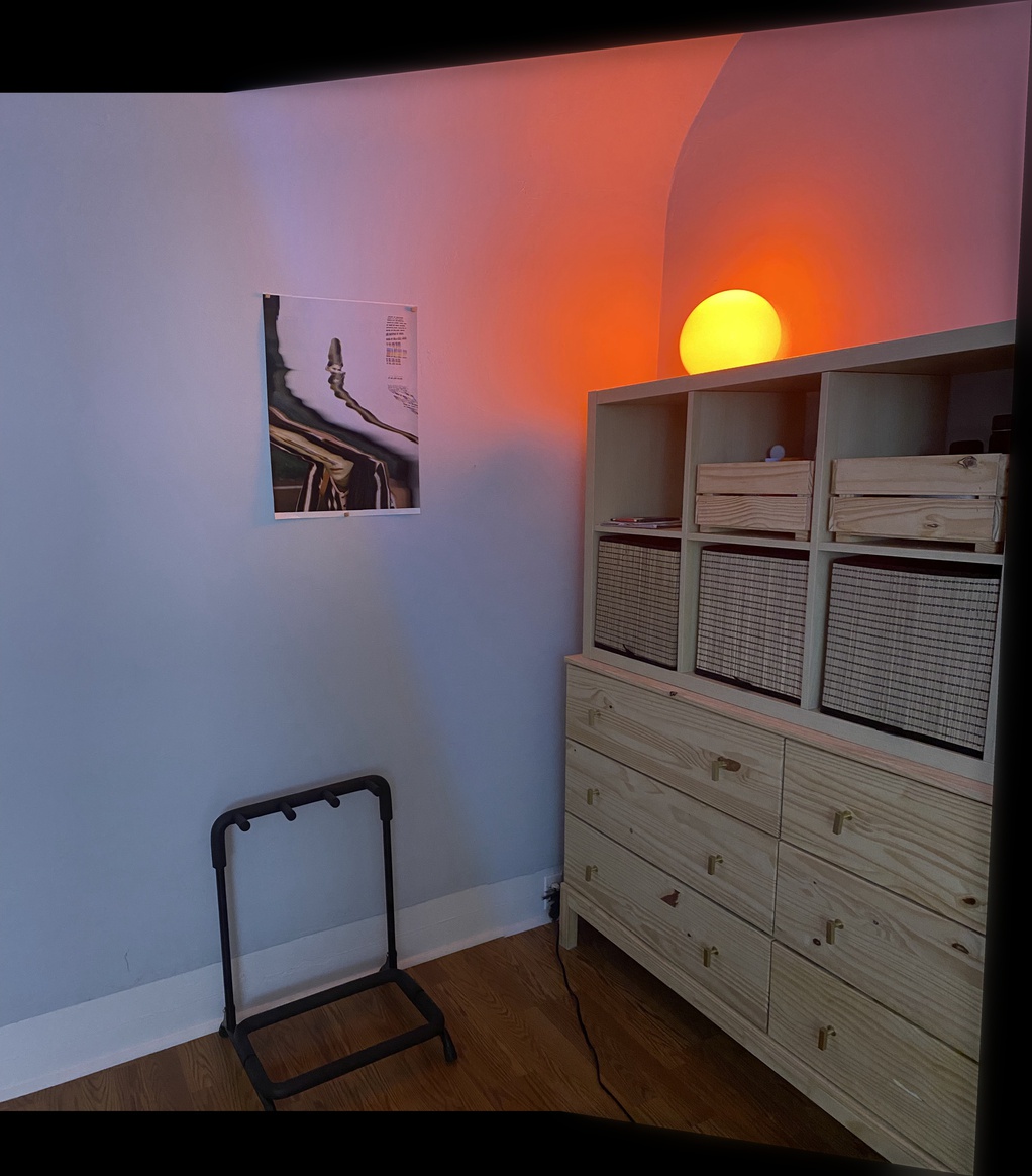
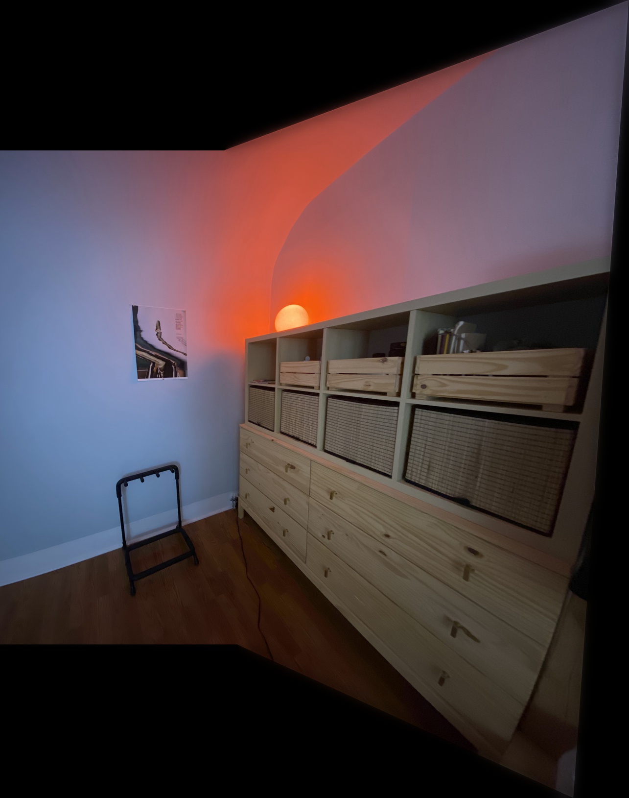
Image warping is very sensitive to fluctuations in the chosen homography points, which makes selecting them a tad tricky. I also initially tried stitching together images that were just barely touching (10% overlap) and this yielded very noisy/unstable results. I enjoyed being able to update and use my seam blending code from project 2 (along with a slew of other helper functions built up for the projects). Visually debugging things is essential, and I updated my plot() image viewer to shrink images before showing them which greatly sped up debugging times for these larger images. Note all images were reduced in size to fit the file zip size limit.
I implemented multi-band blending along with a custom automatic region specifier (as detailed in Mosaics). I also experimented with wide lens imaging, and reported results.