This project explored and put into practice the idea of recovering a homography transformation matrix, which is a three-by-three transformation matrix with eight degrees of freedom (the bottom right matrix value is set to one). The steps taken to recover the homography transformation matrix are explained in more detail under the “Recover Homographies” section. Using the computed homography transformation matrix, we can warp each respective image so that identified image features from the source will match the destination’s feature locations. After warping, the images are ready to be blended to produce a mosaic. Additionally, another application of recovering a homography transformation matrix and warping an image is image rectification which is used to take an identified planar surface in the image and warp the image to make the plane parallel with our perspective plane of the image which is called “frontal-parallel” in the project spec.
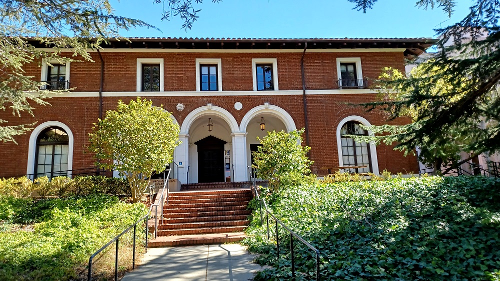
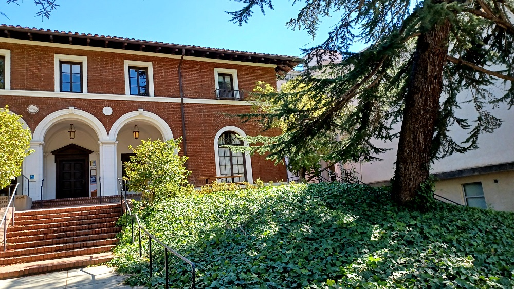
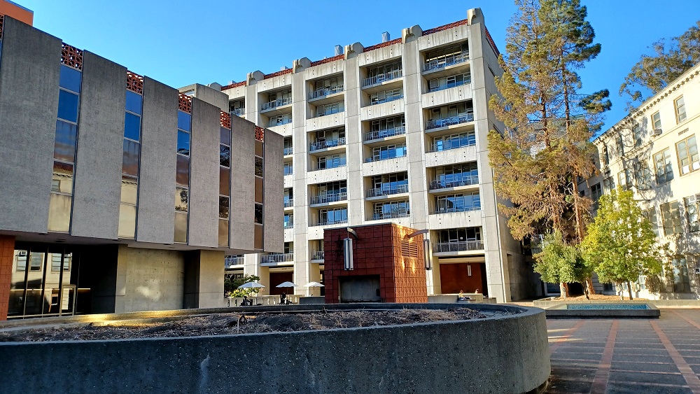
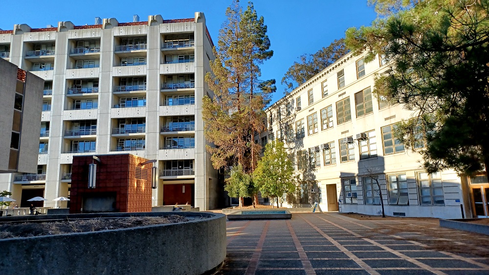
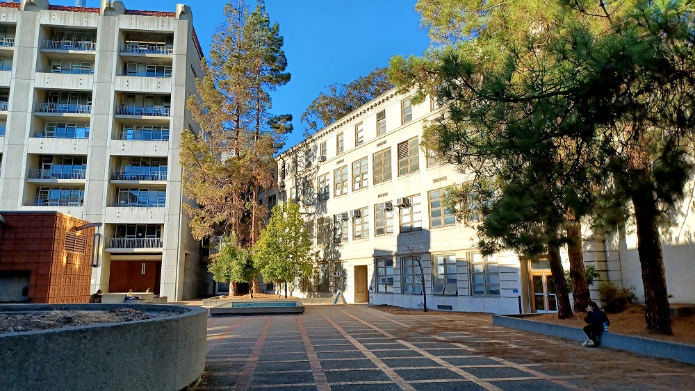
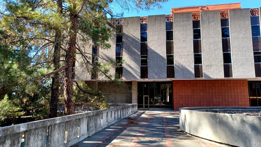
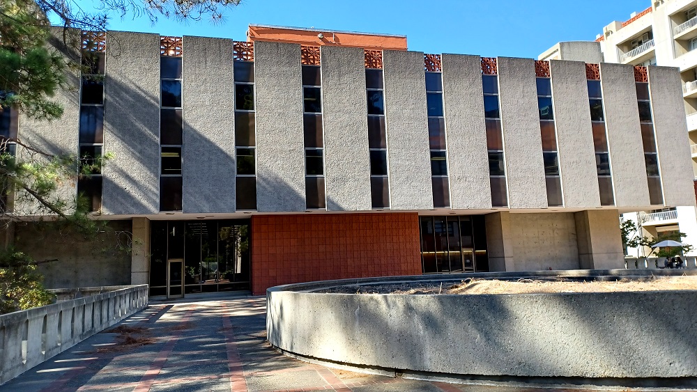
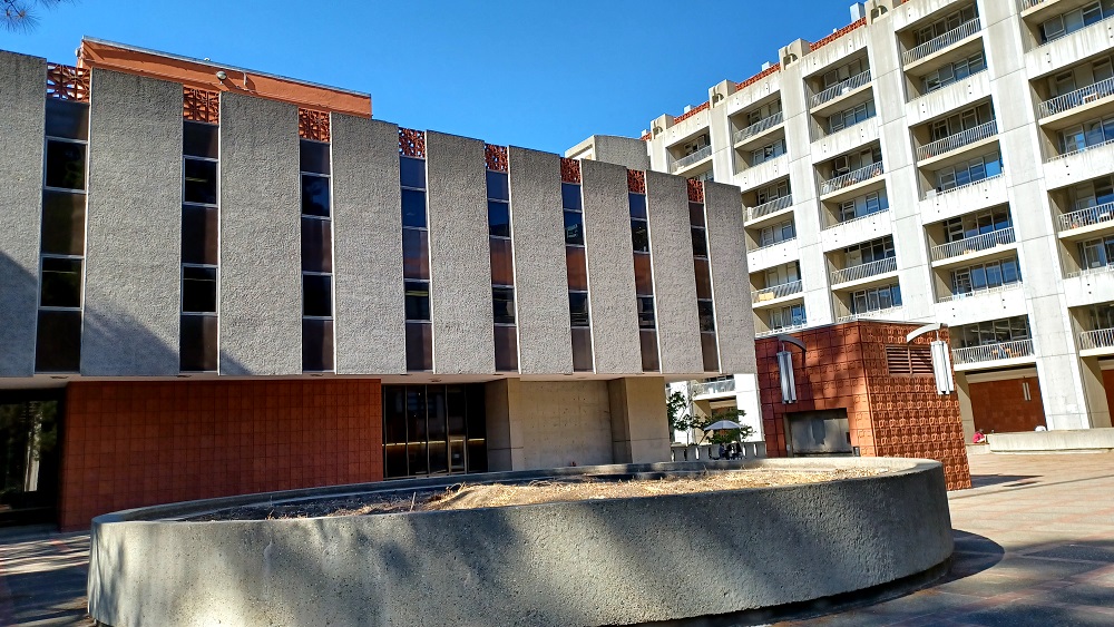
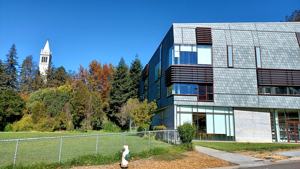
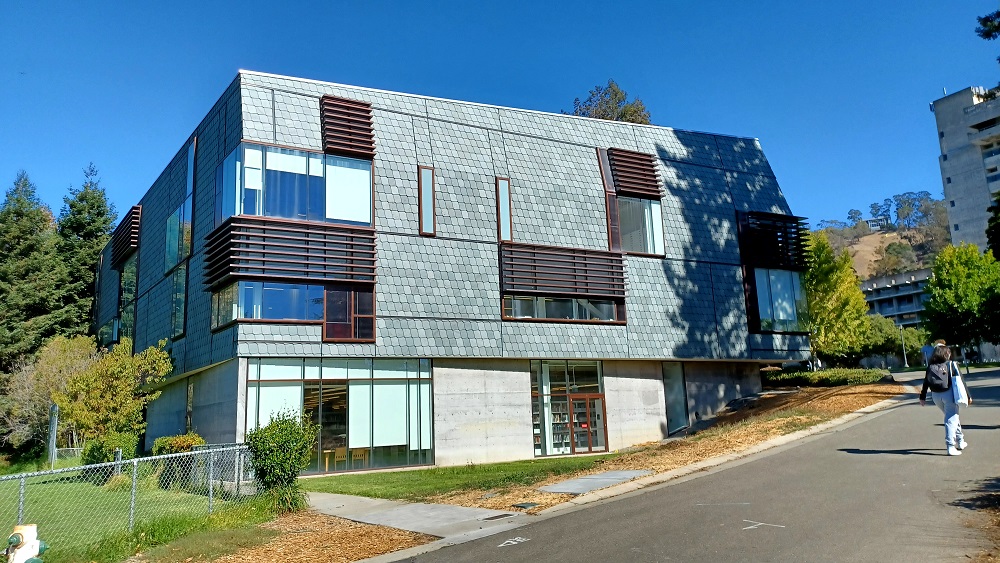
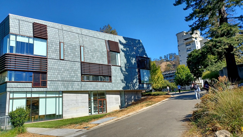
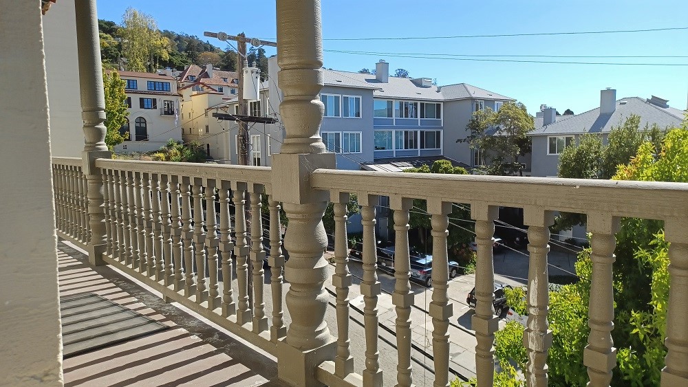
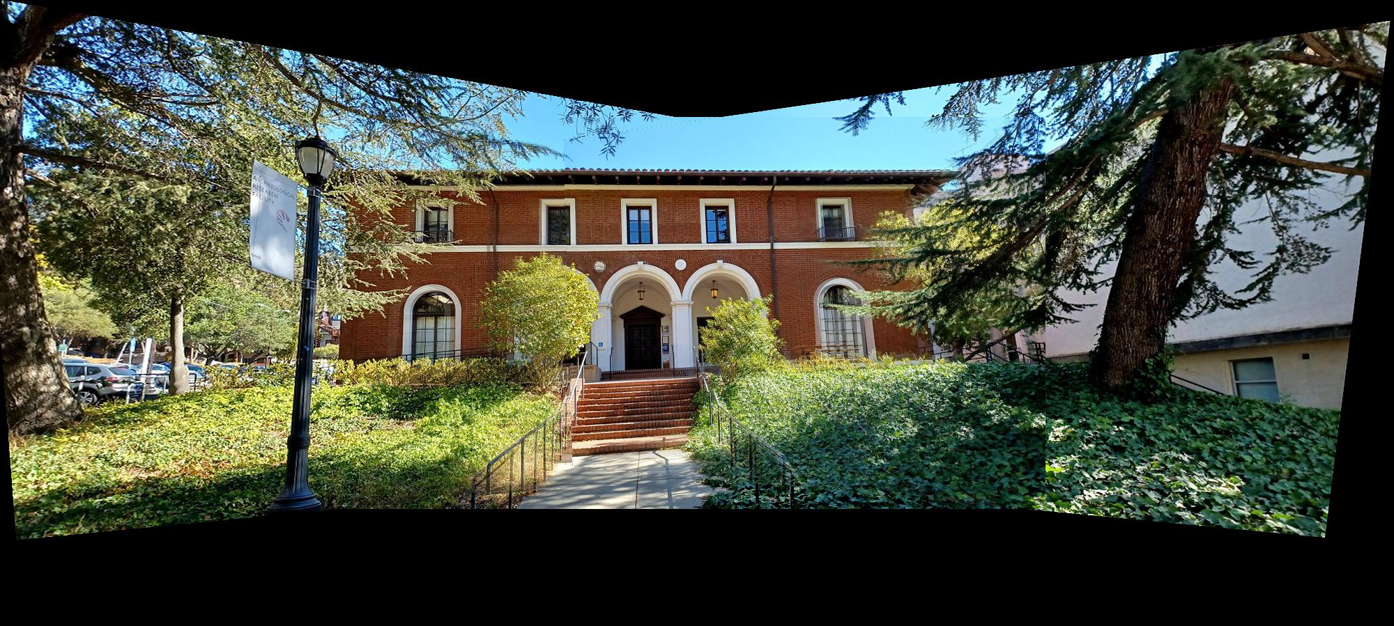
In order to produce the blended mosaics of images or rectify planes in images, we first have to take several digital pictures on which to perform the operations. Below are the digital images I took which will be used in each section. Their use case (i.e. image rectification or mosaics) is identified by the subheading under which they are displayed. Images used for producing each mosaic were taken from a single point of view (as best as possible) and the second image in each mosaic is used as the reference image from which the other two images are warped to match the identified features shared across all images. My code, however, is capable of supporting an arbitrary number of images (see “Recover Homographies” section for details) as long as a reference image is specified, which is used to warp all the other images to the reference feature coordinates.
Images Used for Image Rectification

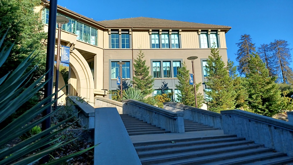
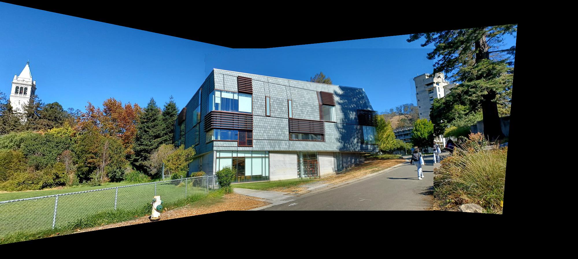
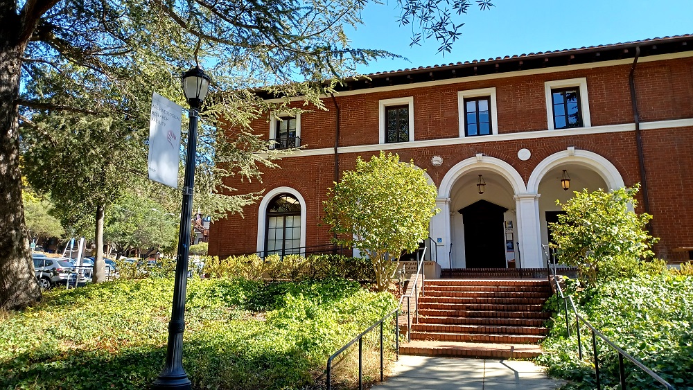
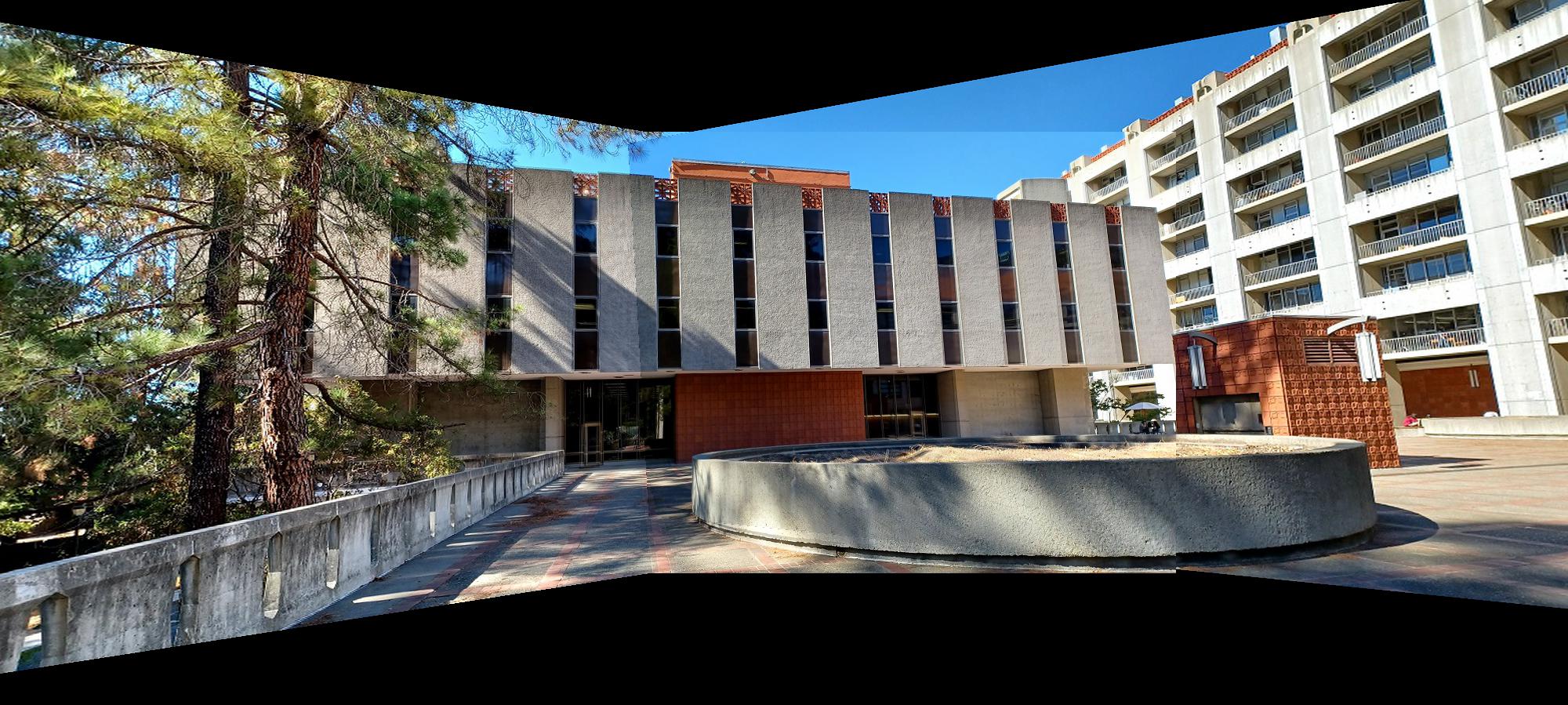
Images Used for Making Mosaics
In order to recover homographies, we need at least four correspondence points to be defined between two images, one being the source image and the other being the destination image into which the homography transformation matrix will warp the pixels from the source image (performed in the “Warp the Images” section). This is because our homography matrix has eight degrees of freedom, and each correspondence coordinate provides two values, an x and a y, so only four points are needed; however, additional points can improve the accuracy of the image warping by computing a better homography matrix since selecting the exact pixel values for the correspondence points between the two images is very difficult. By using more points, the homography is computed using least squares to minimize the error for the homography matrix. Thus, the more points used, the less likely the image warping and subsequent mosaic will be prone to significant errors. I have outlined the steps for computing the homography matrix below which assumes that the first step of manually defining at least four correspondence points on two images has been performed. I found this section to be challenging in rewriting the provided homography transformation equation offered in class into the form Ax=b with x containing the unknowns for our homography matrix.
We begin with the provided transformation equation offered in lecture. The coordinate vector on the right of the equation (p) refers to the source image correspondence points which are being transformed by the homography matrix (H) to produce the destination image’s correspondence points (p’).

We can expand this notation to view the values of the vectors and homography matrix in order to perform further computation. Here, x and y refer to the source correspondence coordinate and x’ and y’ refer to the destination correspondence coordinate. We note that x’ and y’ are scaled by w which cannot be assumed to be 1; thus, in the subsequent computation we will have to account for the w scaling term to extract the true destination points when performing image warping using the computed homography matrix.

From here we expand out the terms by performing matrix vector multiplication and extract three equations.


We observe that the first two equations share the w term which we can substitute into the first two equations as follows:


Expanding out the terms, we get the following:


From our previous assumption, since our homography matrix only has eight degrees of freedom, the i term in the homography matrix can be set to 1. This simplifies our equation by substituting 1 for the value of i:


Isolating the x’ and y’ terms now on the left side of the equation, we get the following two equations:


We can now rewrite these equations in matrix vector notation that conforms to the Ax=b format we desire. The resulting matrix and vectors are as follows:

The subscripts used in the above expression represent the correspondence coordinate to be used. Since we need a minimum of 4 points, then in the above notation, the values for the first point (x1, y1) should be appropriately substituted as well as for the second point (x2, y3), the third point (x3, y3), and the fourth point (x4, y4). However, we want to be able to process more than four points and compute least squares when determining the values of our homography matrix which are contained in the x vector. Thus, the above expression is generalized to accept n defined points, as denoted with the subscript n following the ellipses in both the A matrix and b vector. We solve for the unknown homography variables as follows. I will use the abbreviated Ax=b notation for the following computations.
We start with the above defined matrix vector expression:

Where A is the n by 8 matrix shown above, x is the vector which holds the unknowns for our homography matrix for which we are solving and b is a n by 1 vector that holds the destination x’ and y’ coordinates that are associated with each linear equation. We first multiply both sides of the equation with the transpose of the A matrix to produce a square matrix that is invertible (this is important for the next step)

We then multiply both sides by the inverse of the resulting matrix from the product of A with its transpose. The matrix is invertible since we multiplied A with its transpose. This will leave the identity matrix on the left side of the equation, isolating the x vector of unknowns and allow us to compute what the values of those unknown variables are given n correspondence points.

From here, we simply place the corresponding values in the found x vector into the appropriate locations for our homography matrix and return H (our homography transformation matrix). This is the procedure I implemented in my computeH function which returns the homography transformation from the correspondence points in image1 (the source) to image2 (the destination).
Now that we have computed the homography transformation matrices for each image, or only a single image as is the case for image rectification, we can warp the images given the homograph transformation matrix. In its current format, the homography transformation matrix will translate coordinate values from our source image, the input image, to some new warped coordinates which I will call the destination image. This would result in forward warping the image; however, in order to avoid aliasing on the warped image, my warp function first finds the inverse of the homography transformation matrix so that I can inverse warp the image and use interpolation to sample the original image for each warped pixel’s coordinates.
More specifically, my warp function first begins by initializing three new canvases, for the red, green, and blue color channels of the warped image, that are of the same dimensions as the input image. Then for the three color channels of the input image, I define interpolation functions each using RectBivariateSpline. I then get all of the pixel coordinates in the image in order to warp each of those pixel coordinates and perform the subsequence sampling of the original image. Before doing so, I find the inverse of the homography transformation matrix such that the transformation matrix will now convert the pixel values on the warped image’s canvas to the appropriate pixel values to be sampled from the original source image (before inverting the transformation matrix, it would take the pixel coordinates of the original source image and convert them to the coordinates associated with the warped image). The result of inverting the homography transformation matrix to perform inverse warping is more clearly shown in the following equations.


Inverting and applying the homography transformation matrix on each pixel coordinate of the warped image canvas, I proceed to sample the original image using the defined interpolation functions given the transformed coordinates. The sampled pixel values are then recombined to form the warped color image which is returned by the function. Additionally, my warp function can also return the mask associated with the warped image, or a black box on the white canvas representing where the warped image lies on the mosaic frame. This is helpful when blending the images together to form the mosaic.
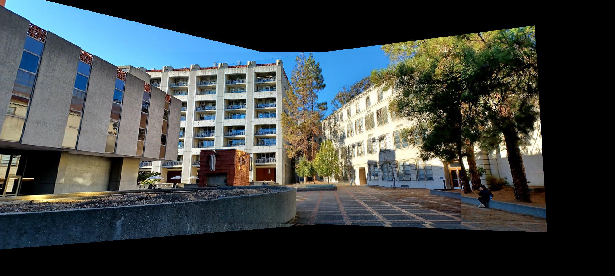
The warped images along with their alpha masks for each of the mosaic images I used are displayed below to demonstrate that the homography transformation matrix and the warping function are working as intended.
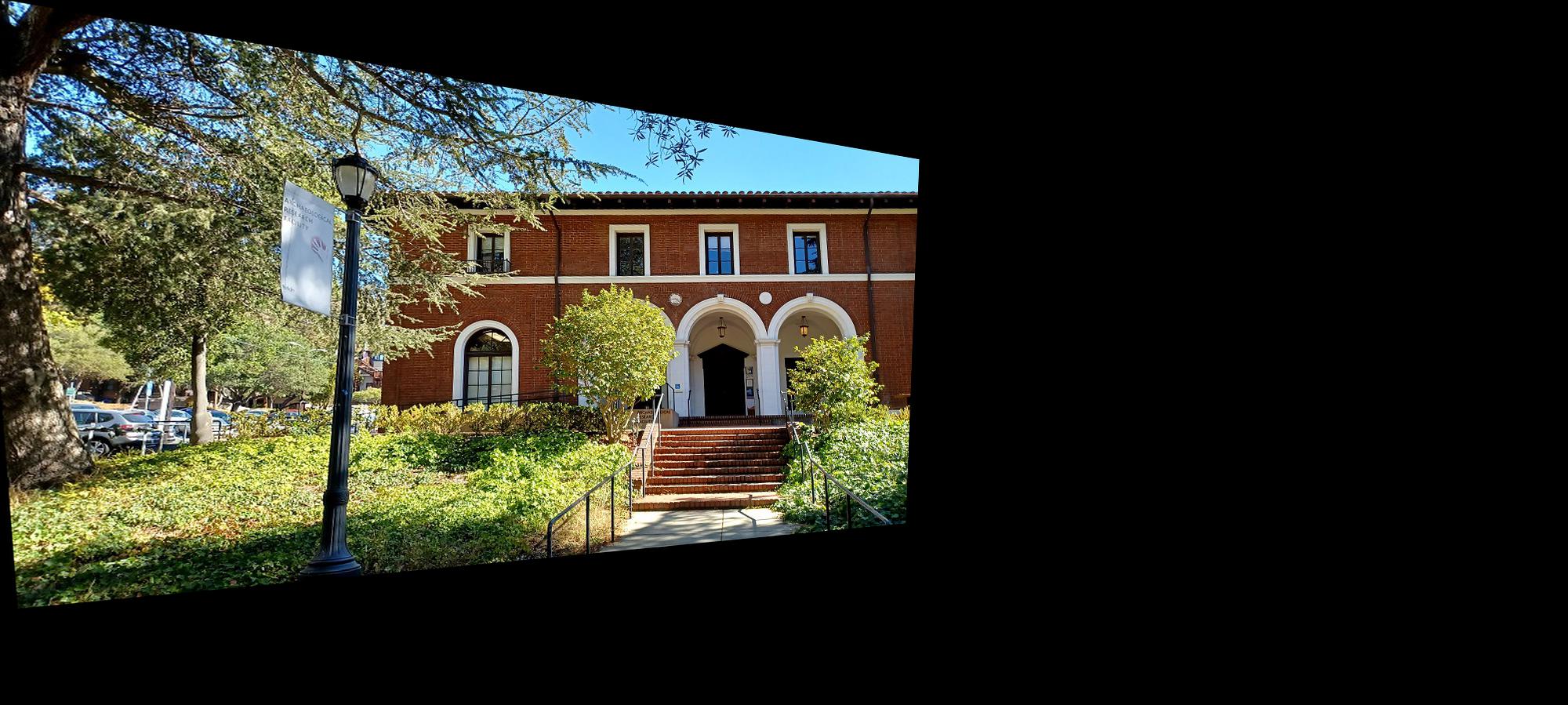
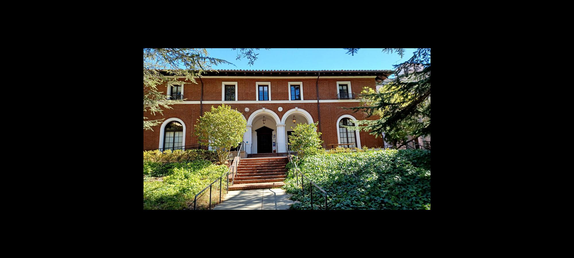
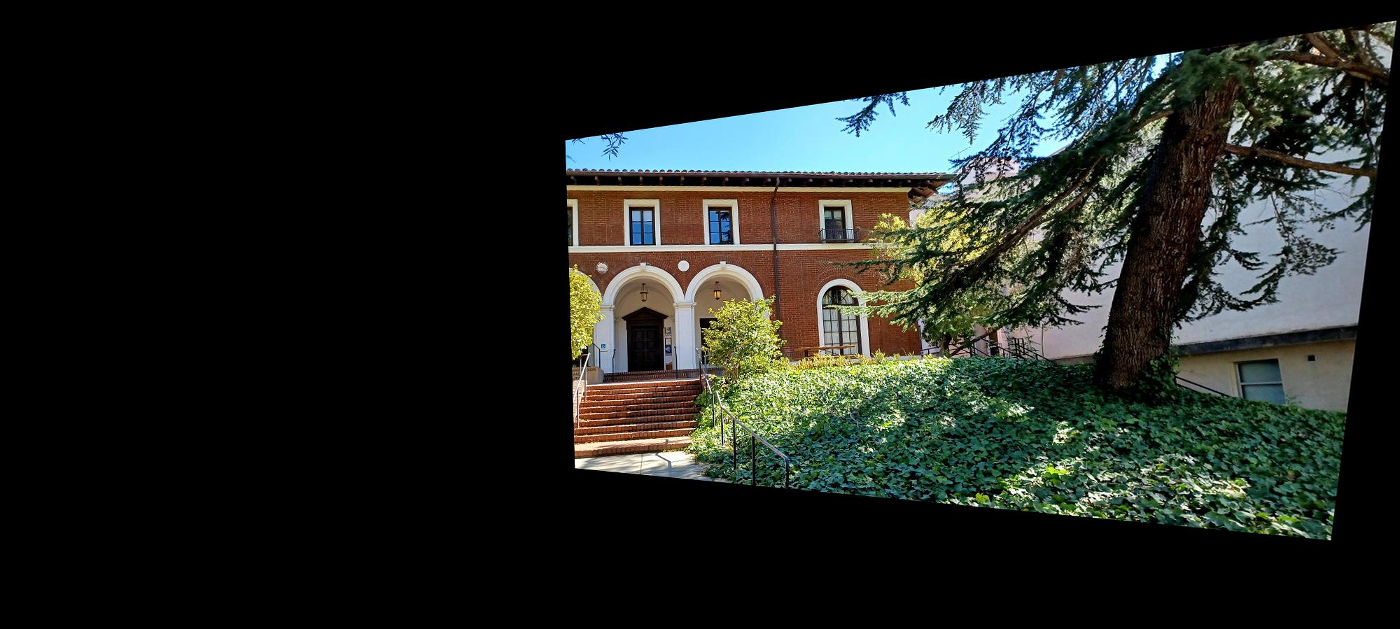


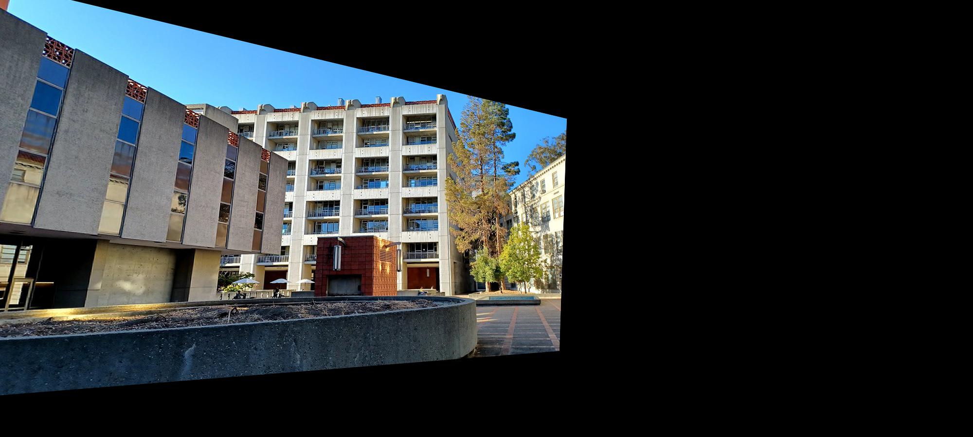
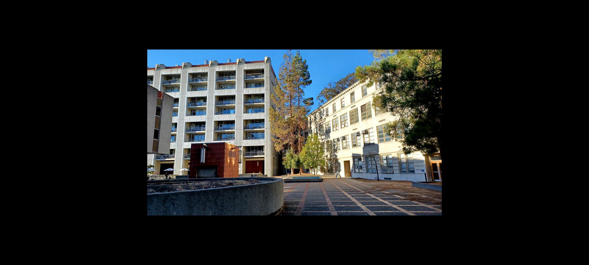
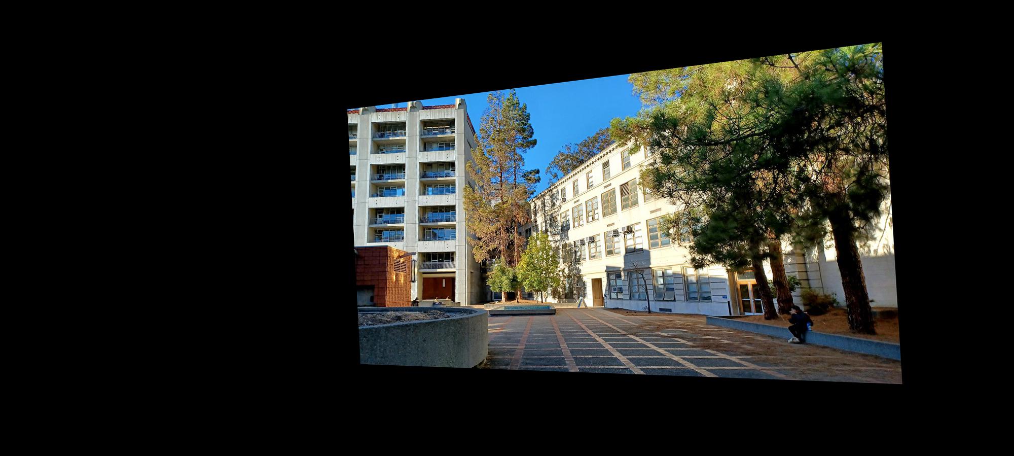


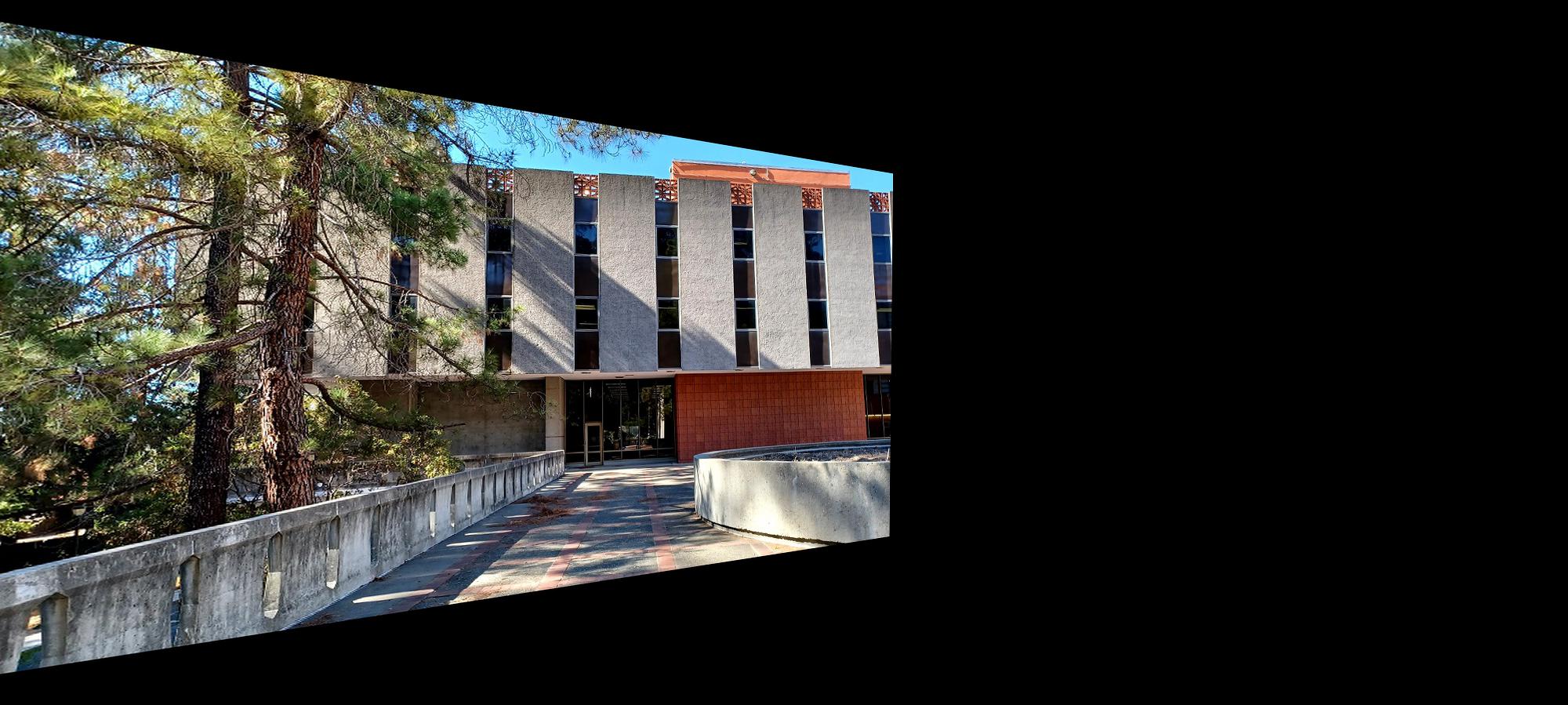
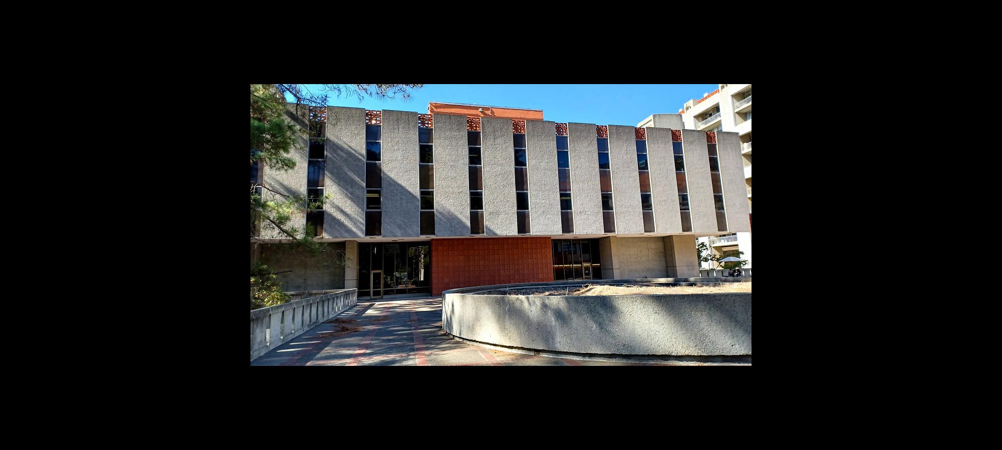
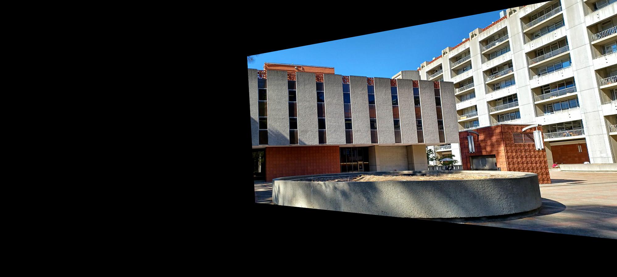


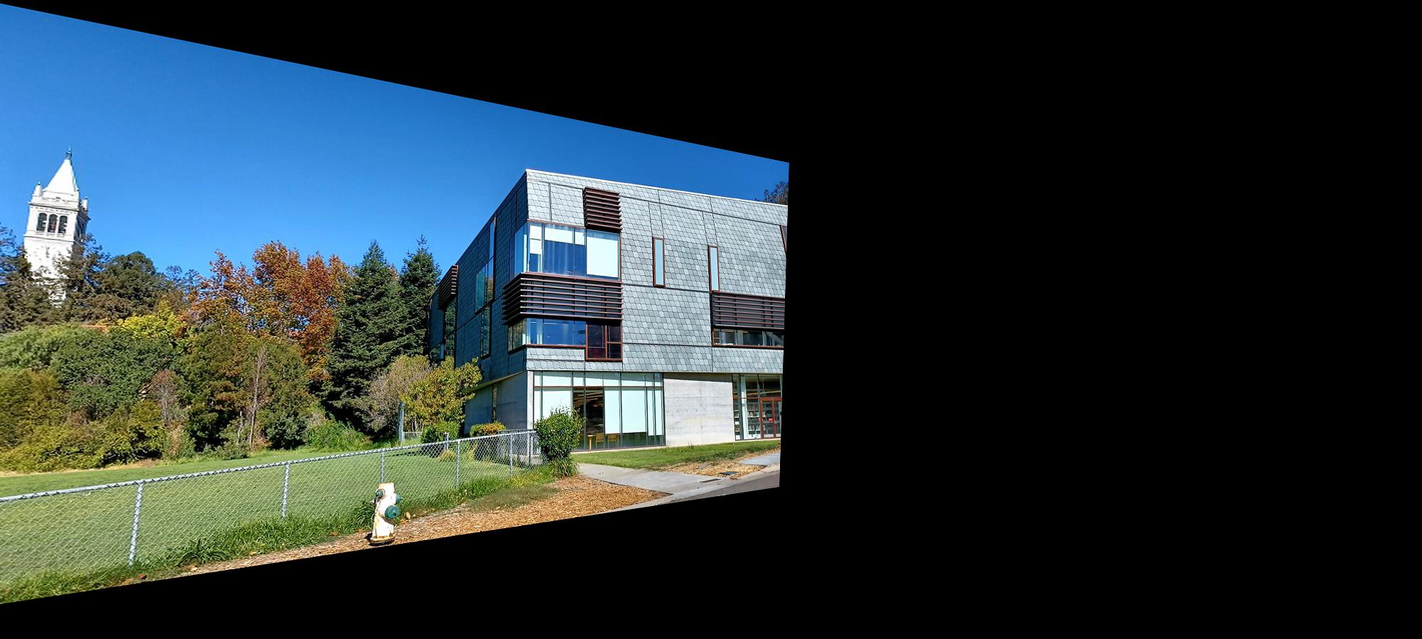
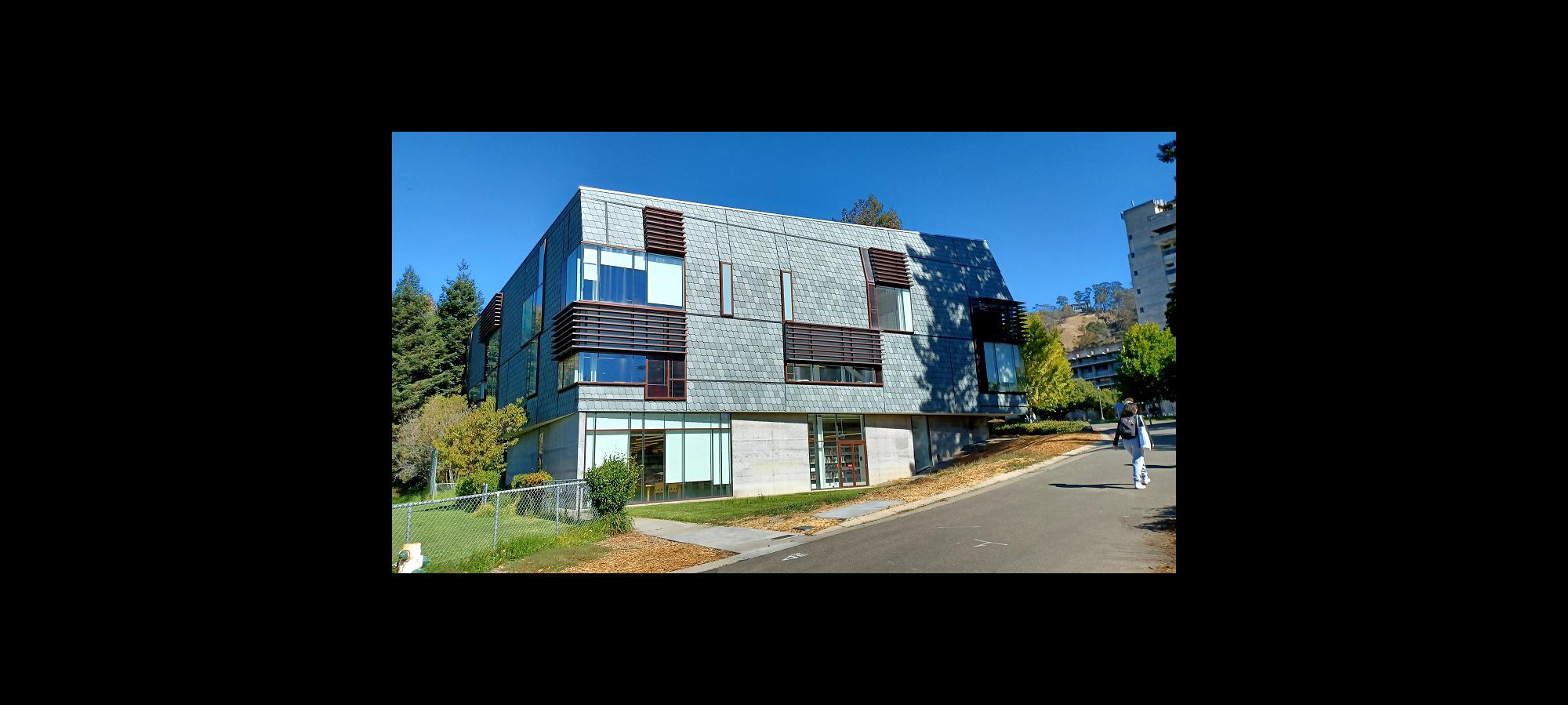
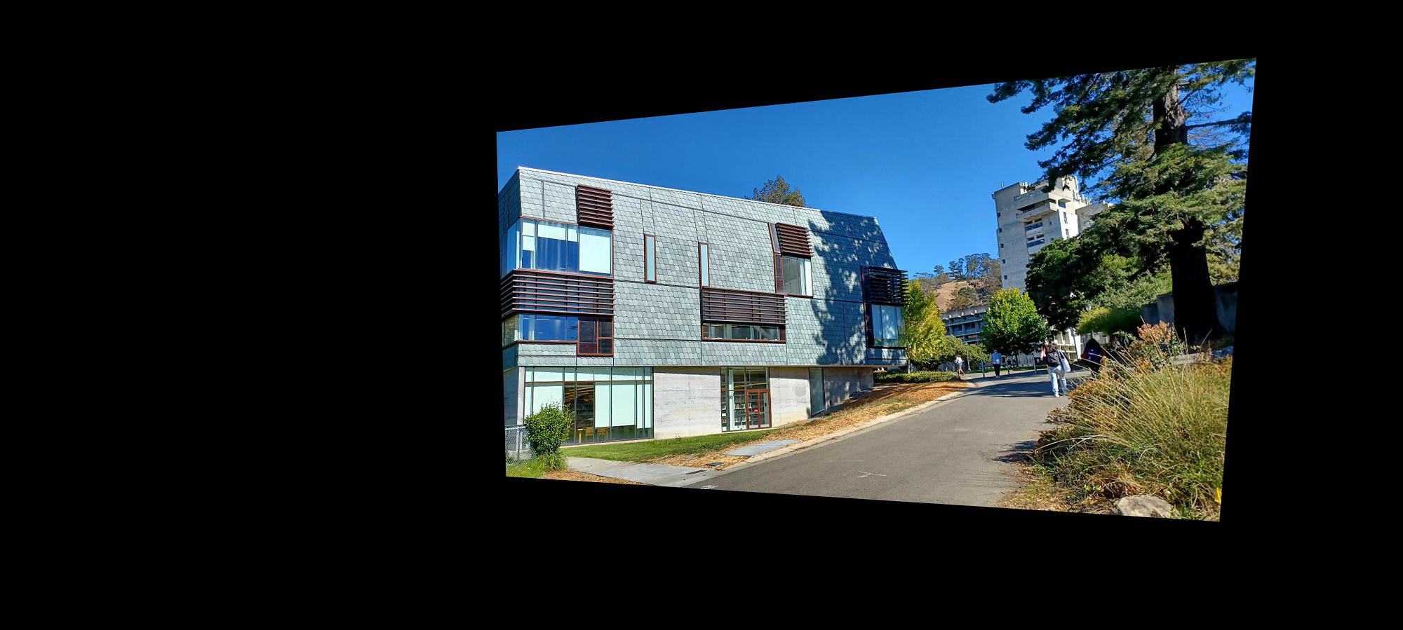


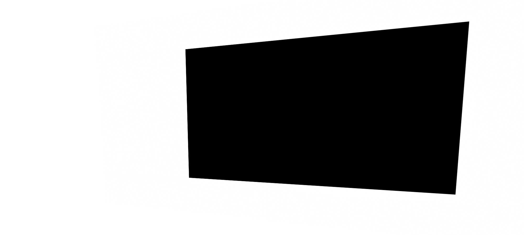
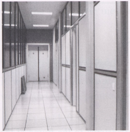
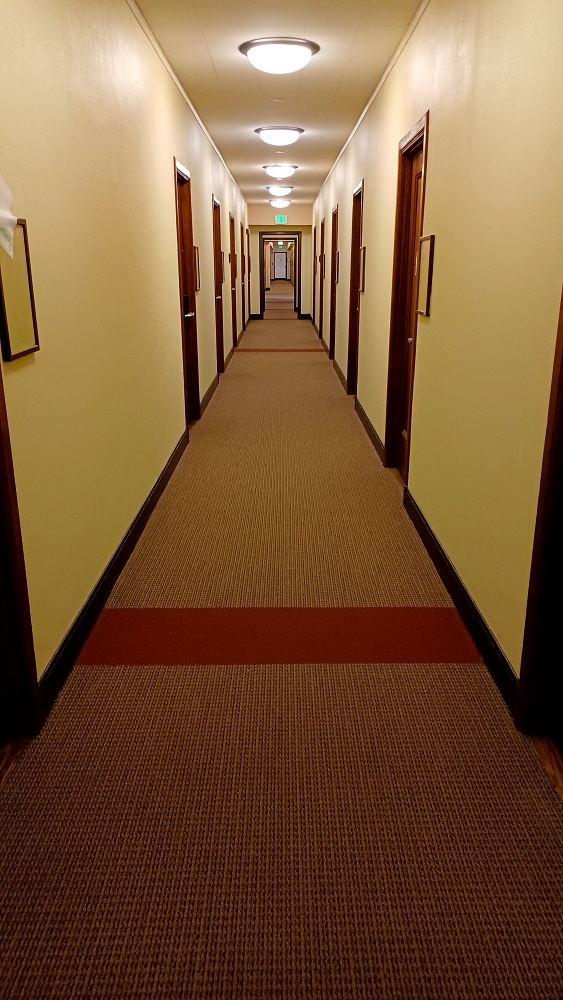
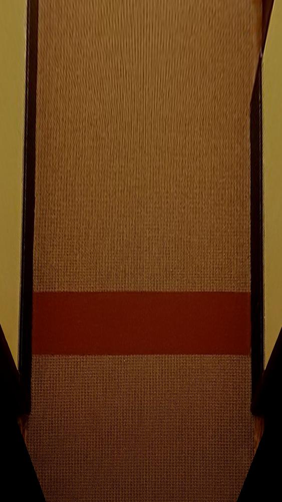
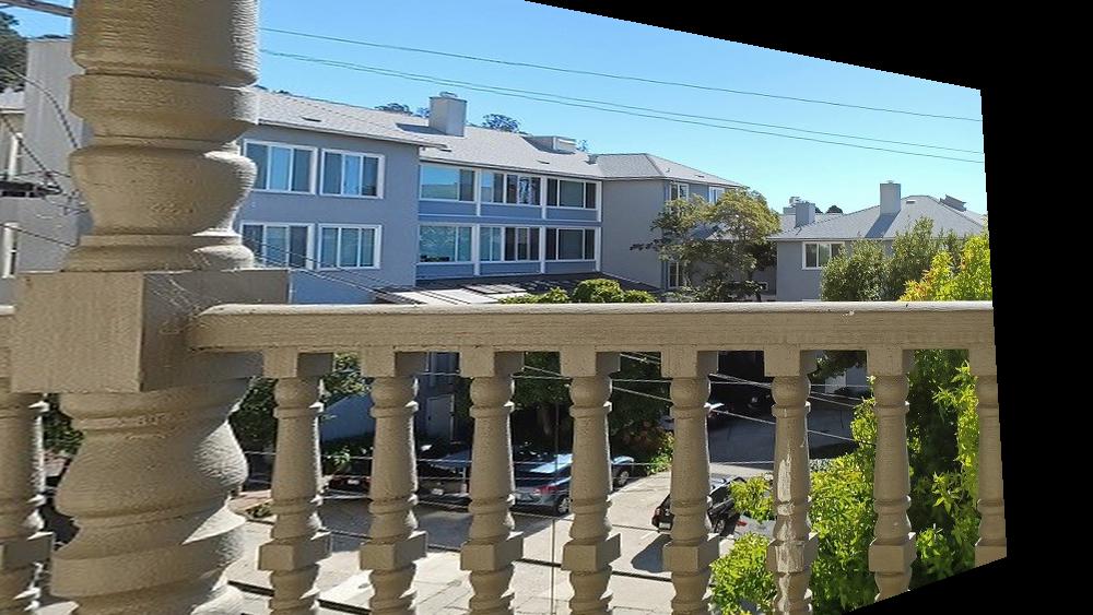
Image rectification uses the same functions we built for finding the homography transformation matrix and warping an image using that transformation matrix but instead of defining correspondence points between two images, we identity a plane in the input image which we want to transform such that the plane in the image is now parallel with the image plane. It helps to know the geometry of the identified plane since the coordinates used to compute the homography transformation matrix are determined manually based on the anticipated geometry of the selected plane. For example, one of my rectified images was that of a hallway which was a carpet with rectangular patches on the ground. I know the rough dimensions of the rectangular patch and can then define the rectangular coordinates with which to compute the homography. This results in a warped image with the carpet feature plane parallel to that of the image plane. It also creates the perspective that we are now looking down on the floor rather than down the hallway even though a separate picture was never taken. Below are a couple of the images that I rectified.
I first began with an input image which we saw in lecture. This was my sanity test-case to make sure that the homography and warping functions were working properly and they did successfully produce the output image from lecture.

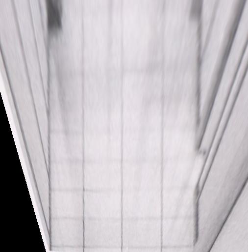
I then rectified the hallway image which I explained above, using the burgundy carpet patch as the rectangular plane on which I was going to rectify the image. The result seems very convincing as if the picture was taken facing down on the floor rather than looking down the hallway, although the black corners on the bottom of the image due to lack of information break the illusion. We can also observe that the pixels towards the top of the rectified image appear blurrier, in the original image, this was part of the hallway further away from the camera, so less detail was captured.
The second image I rectified was taken from a balcony on an angle. I decided to make the railing posts the plane on which to rectify. The results are viewable below.
In this section, we take the warped images previously computed along with their warped alpha masks and combine the images to produce a mosaic. For my implementation, I applied a weighted averaging over the regions of the mosaic where the images overlapped as to make the transition between the two images less abrupt. I did this by first using the alpha masks for each of the images to determine where the overlap regions where and created a new alpha mask for that overlap region. I then applied a gradient weight on the newly created alpha mask so that the weights of one image would increase from 0 to 1 moving across the overlap region and the inverse was true for the other image in that overlap region. Though the weighted averaging using the alpha masks for each image did improve the overall quality of the mosaic, some of the blended frames are still somewhat visible due to two reasons. The first is the change in brightness of some elements in the scene. Unfortunately, I only have my smartphone as a digital camera and even on its manual picture taking setting, not all of the controls were really manual so image processing was still applied to each digitized image. This resulted in images with different brightness as well as other subtle filters applied to them (some kind of AI image enhancing feature my phone does while saving each image). The second is that not all of my manually-identified correspondence points are perfectly accurate and though I used on average about 8 to 12 correspondence points for each image, there are still some errors which can be visible with slight mismatching of image features. I especially noted this when using objects far away in the scene to define correspondence points, the closer objects in the scene were not matched as well even though the far away objects matched very well. The converse was true when assigning correspondence points to objects close to the camera, they would be aligned very well but objects further away in the scene would then lose some of their alignment. Perhaps this could also be the result of image distortion from my phone’s cheap camera lens which is most likely plastic rather than glass. Below are the original images and the computed mosaic from those images.
I found the image rectification part of this project to be very interesting simply because on some images, the illusion that the picture was taken from a different angle with the camera, like pointing downwards instead of down a hallway, is very compelling. In some cases, taking a high-enough resolution of an image and then cropping the black borders after warping and performing image rectification could seem like a completely different picture.
An important thing I learned from this project is how to compute homography transformations and appropriately apply them to warp images and create a mosaic. Previously, image stitching was not something that I understood very well but seems to have a significant role in imaging technology such as panoramas. It was very interesting to learn about how homographies are used to perform image stitching.