Overview
In the first part of this project, we used homographies to combine images into paronamas.
A-1 Shoot the Pictures
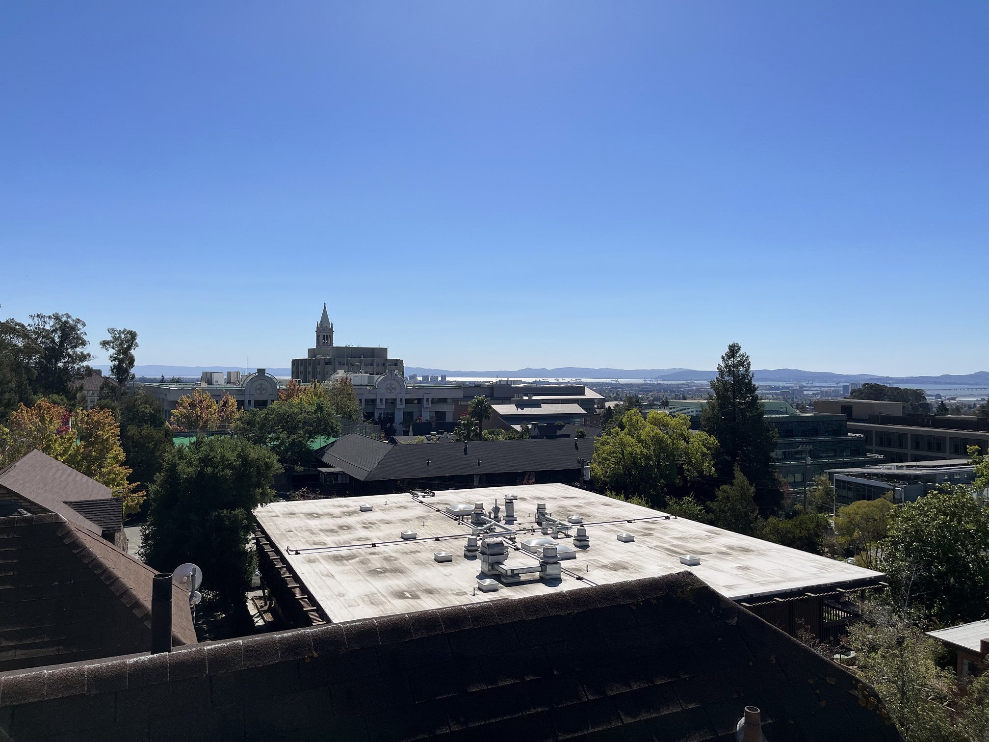
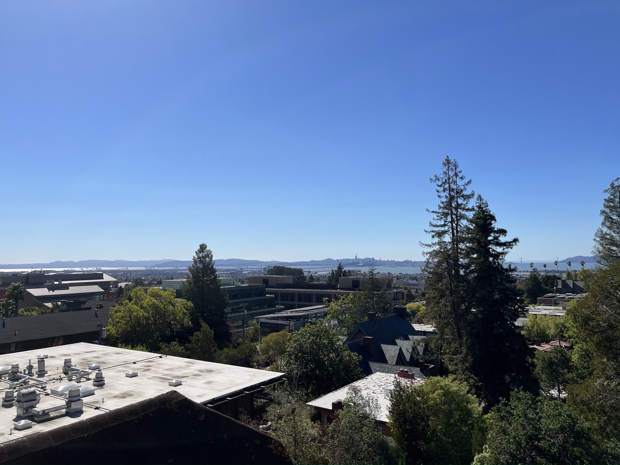
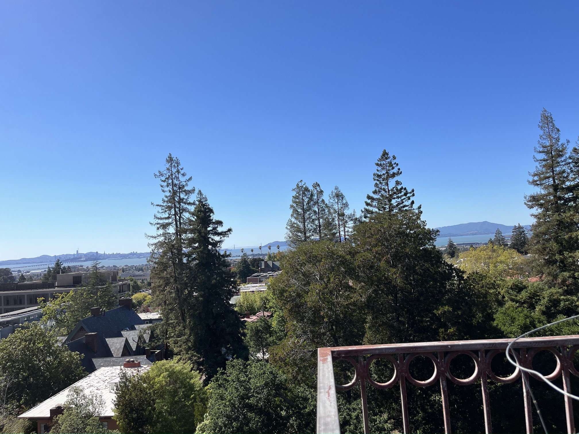
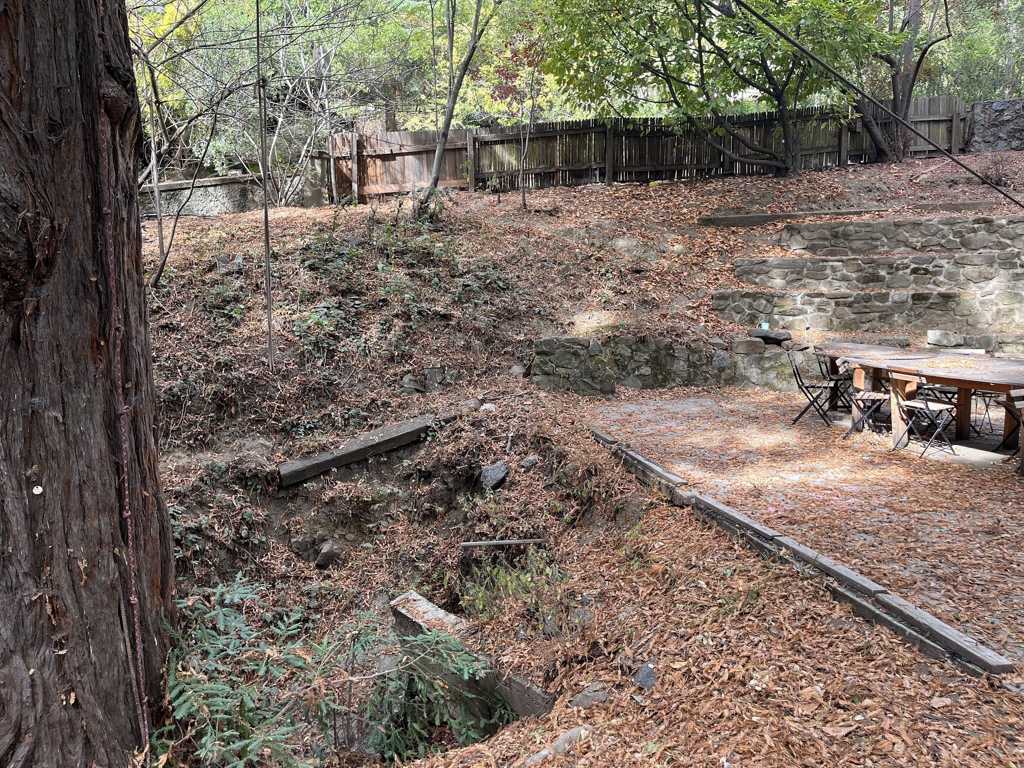
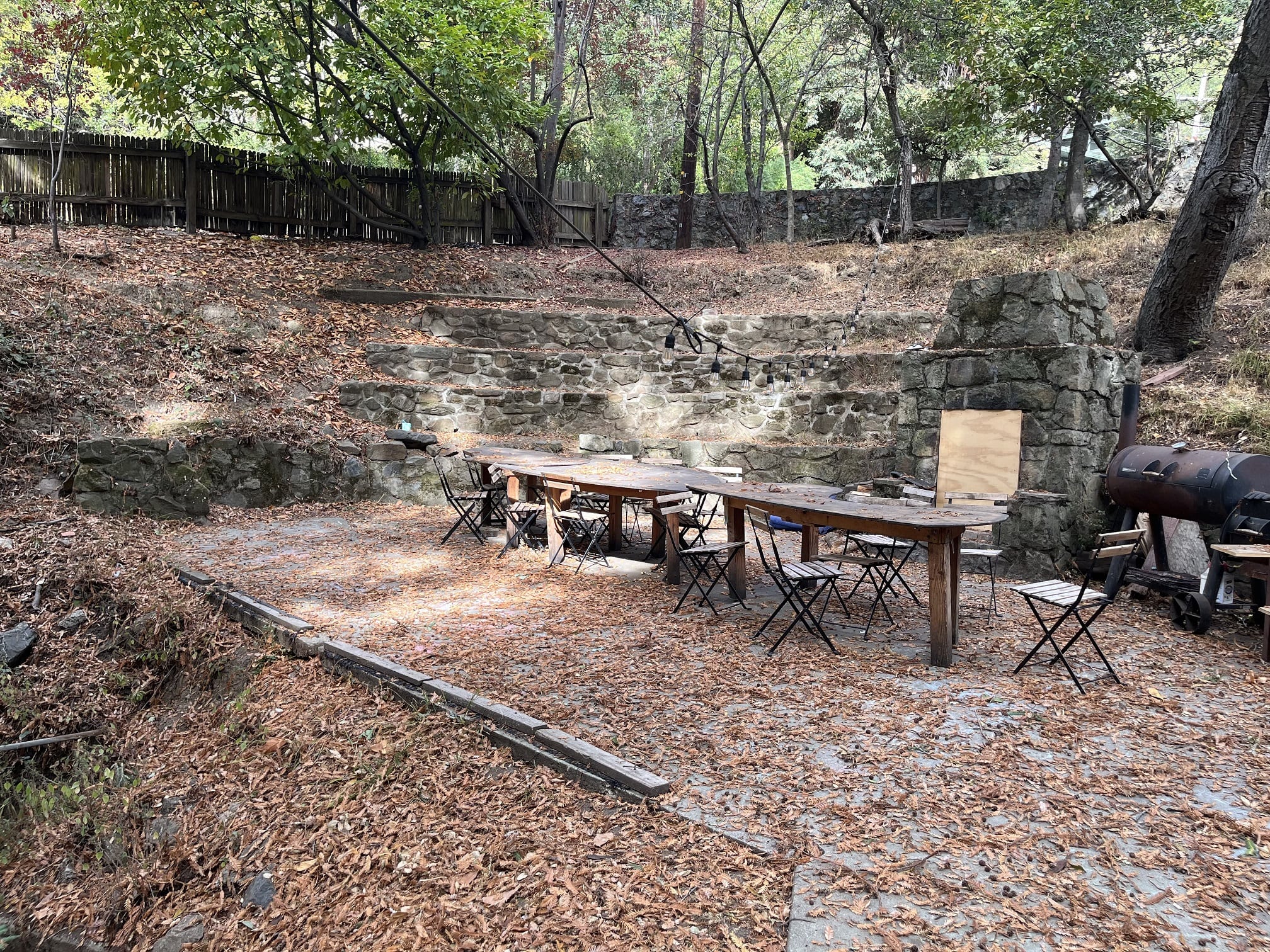
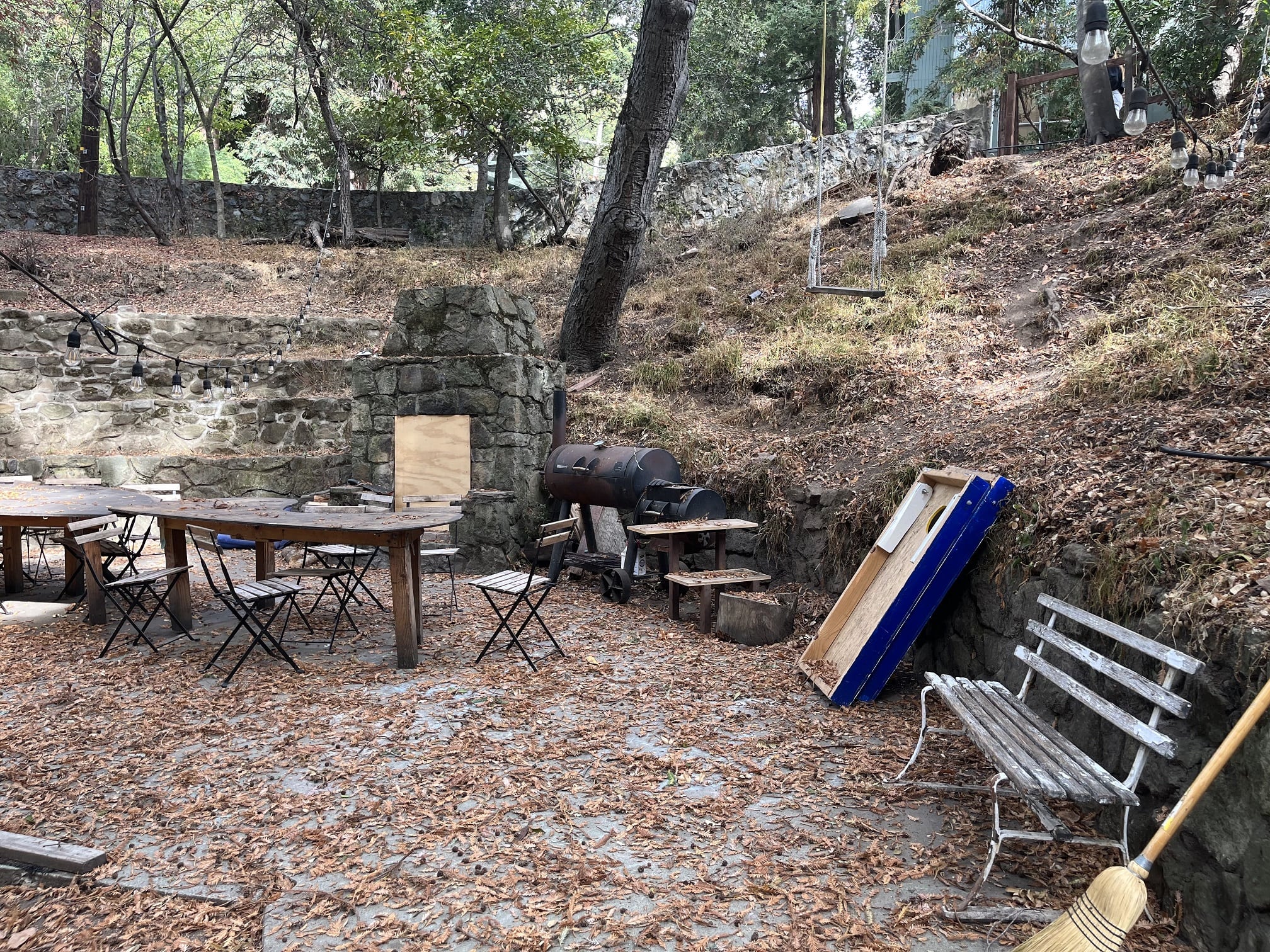
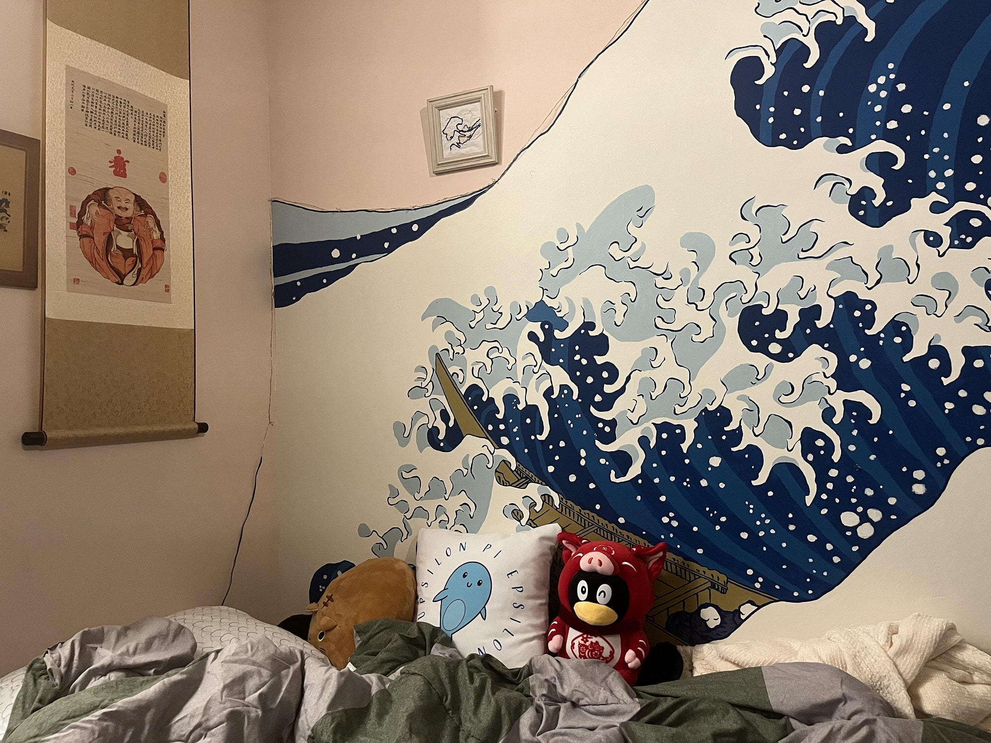
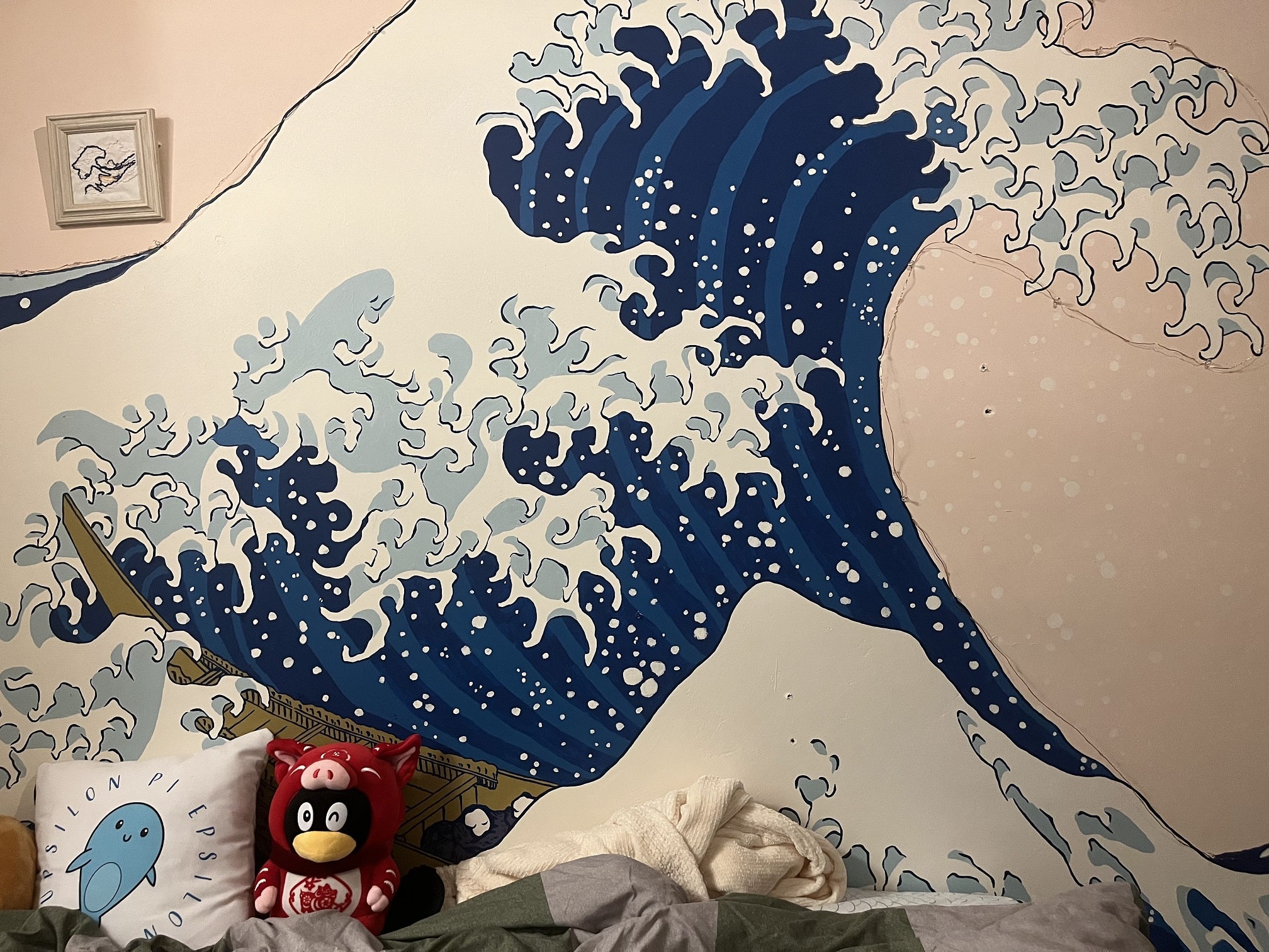
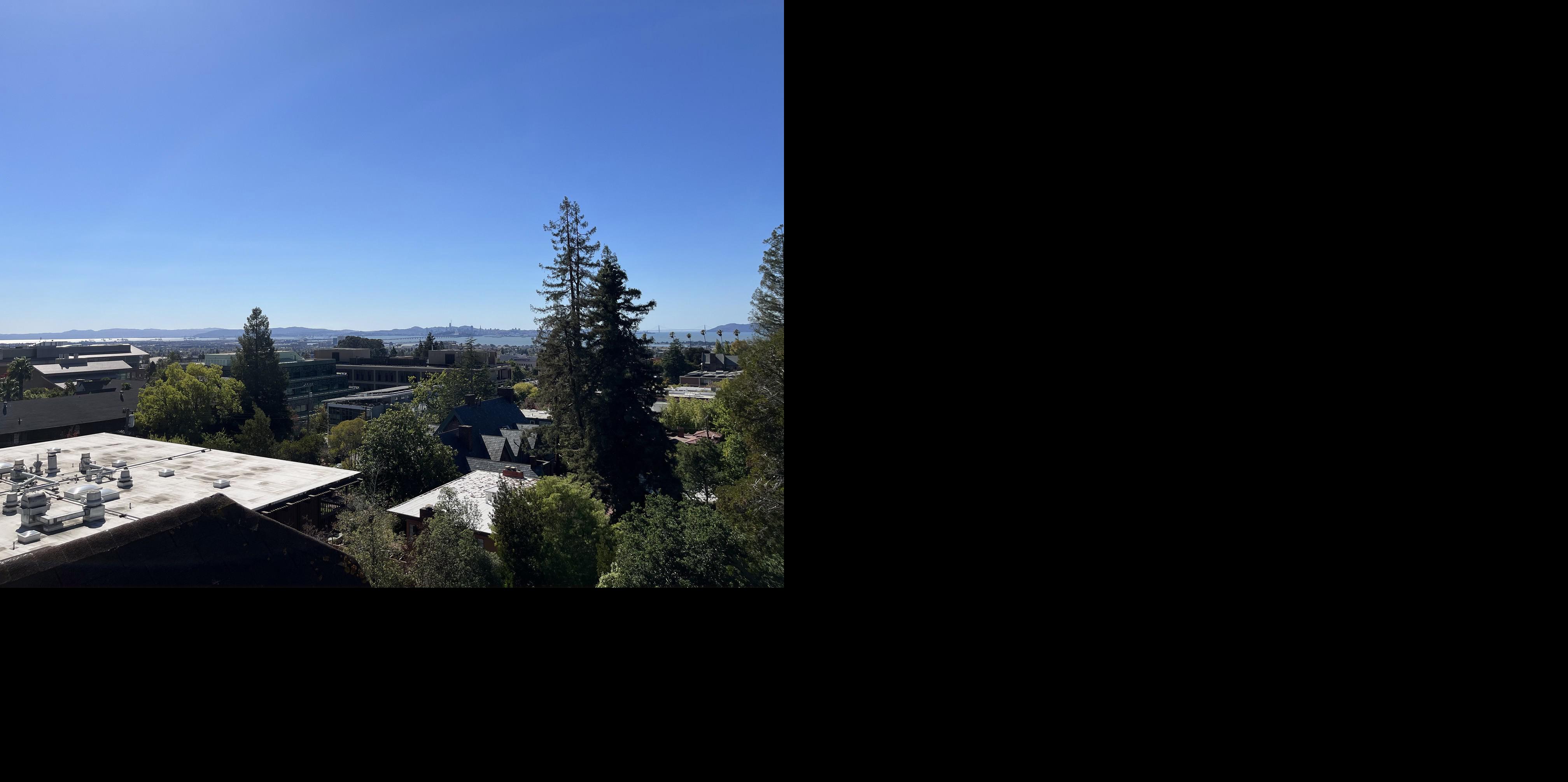
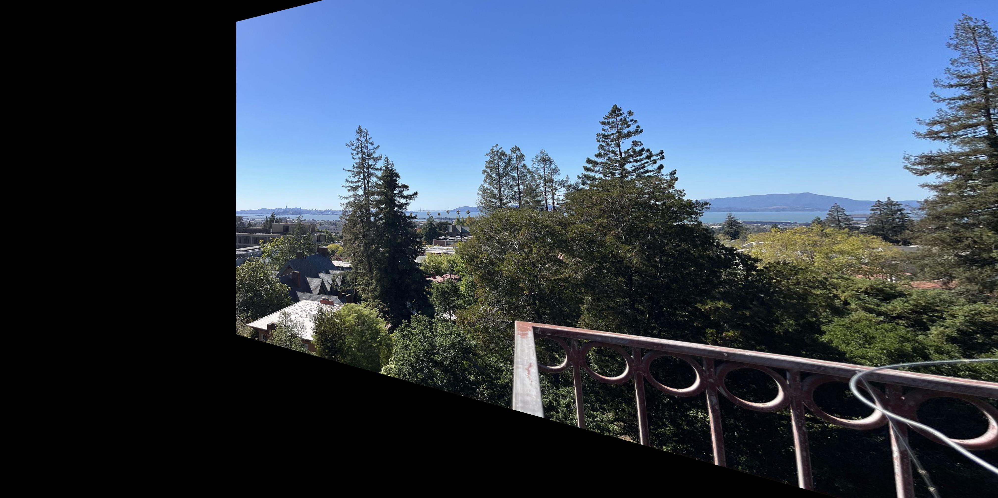
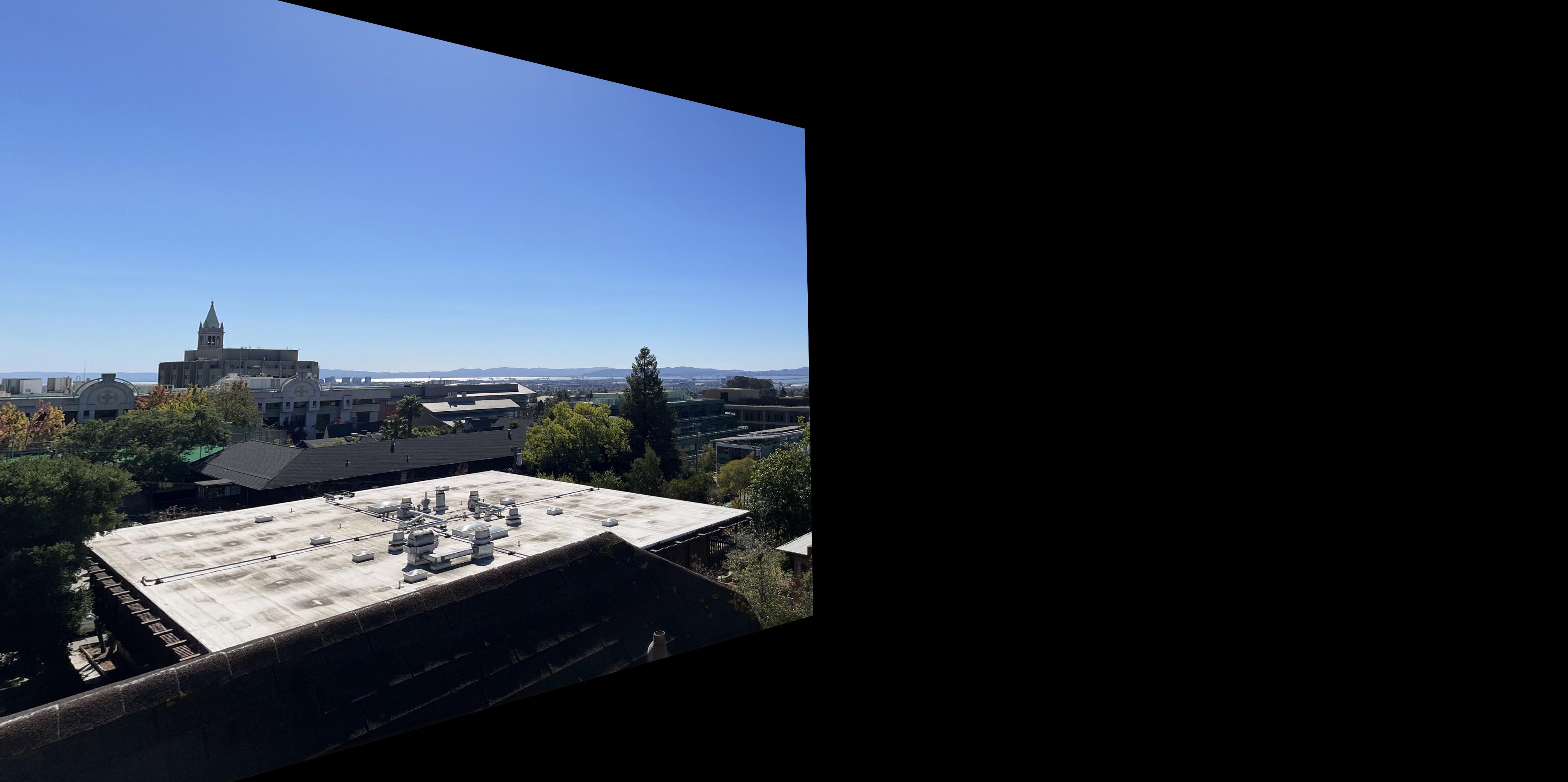
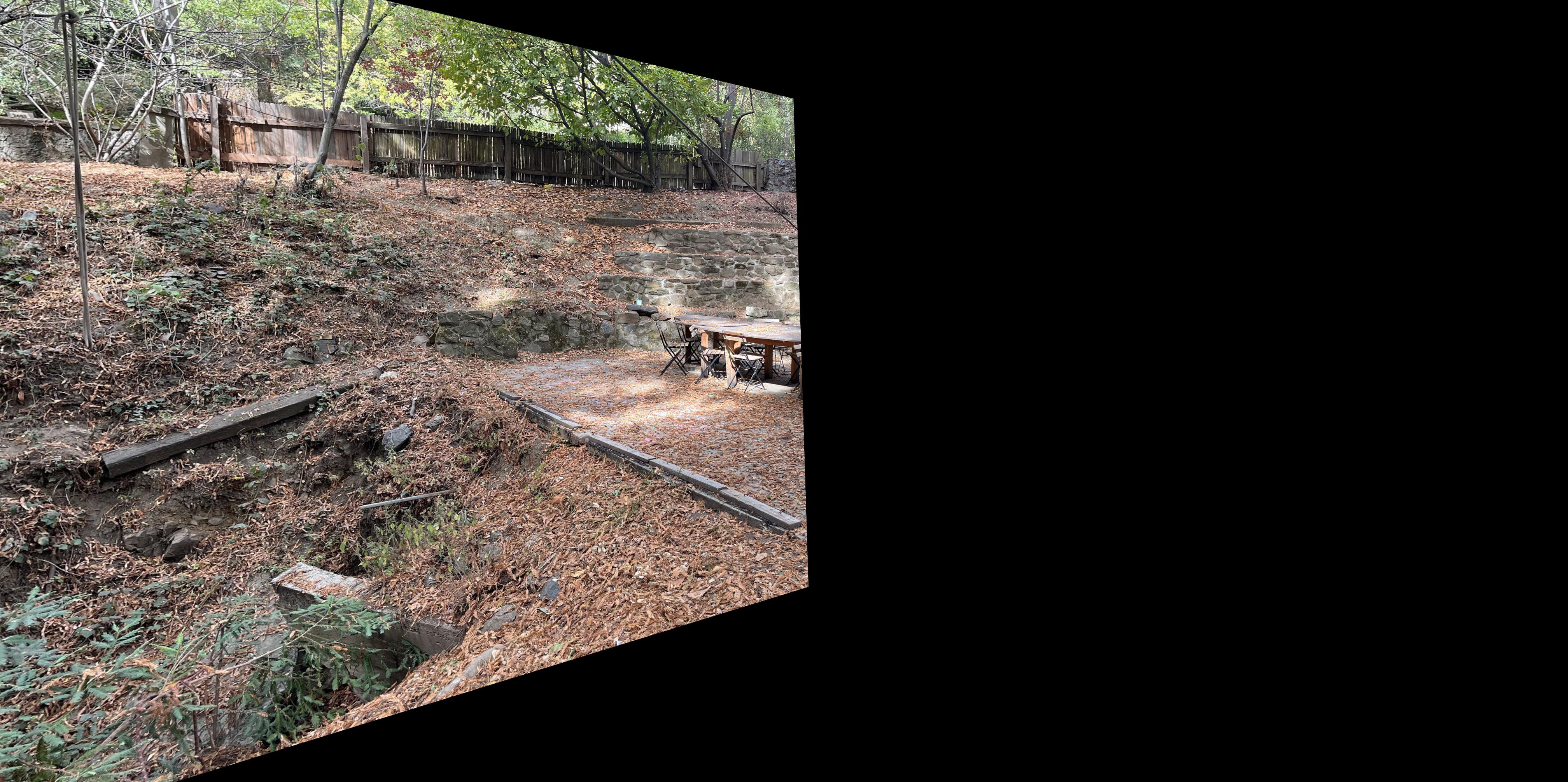
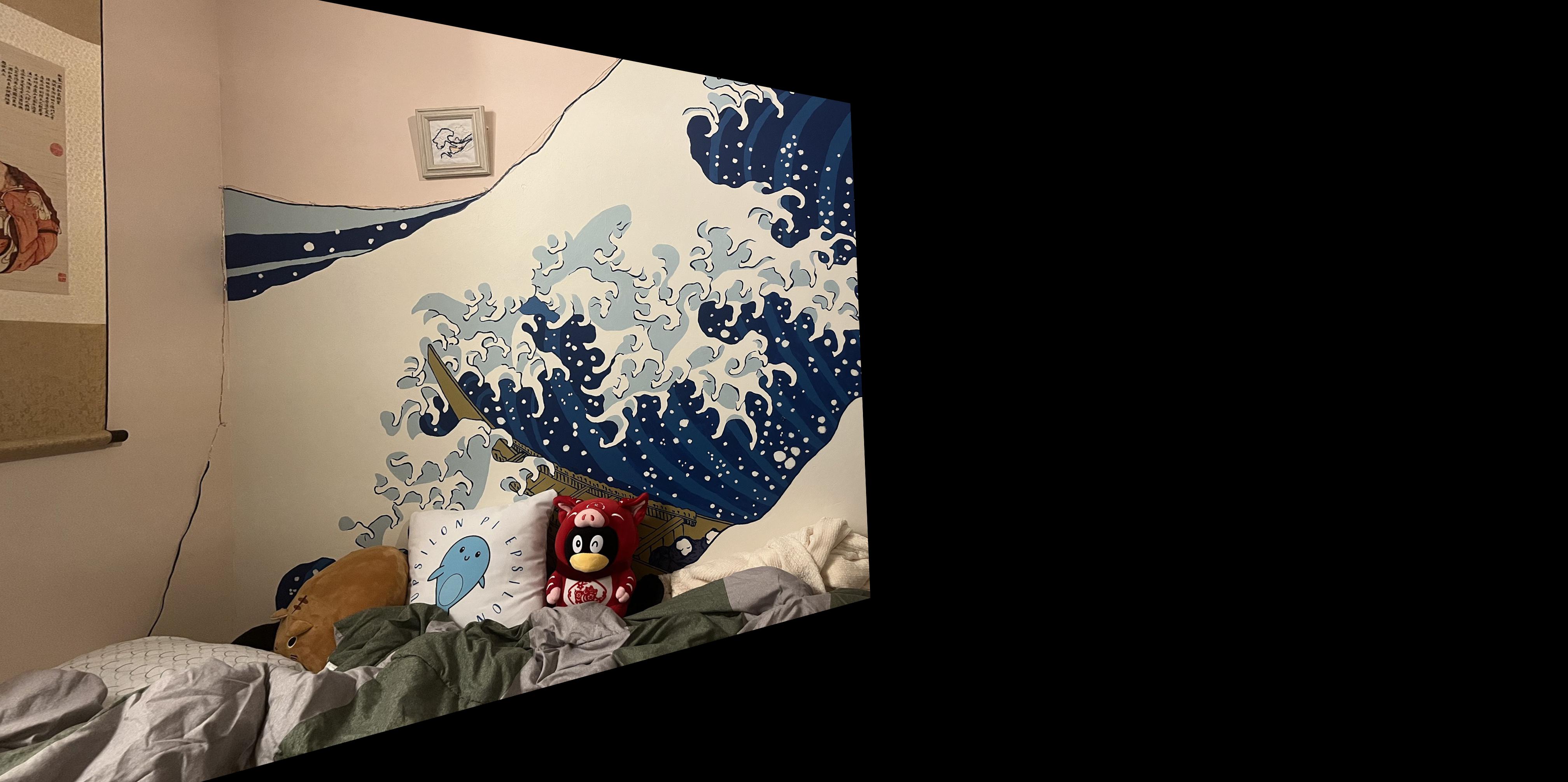
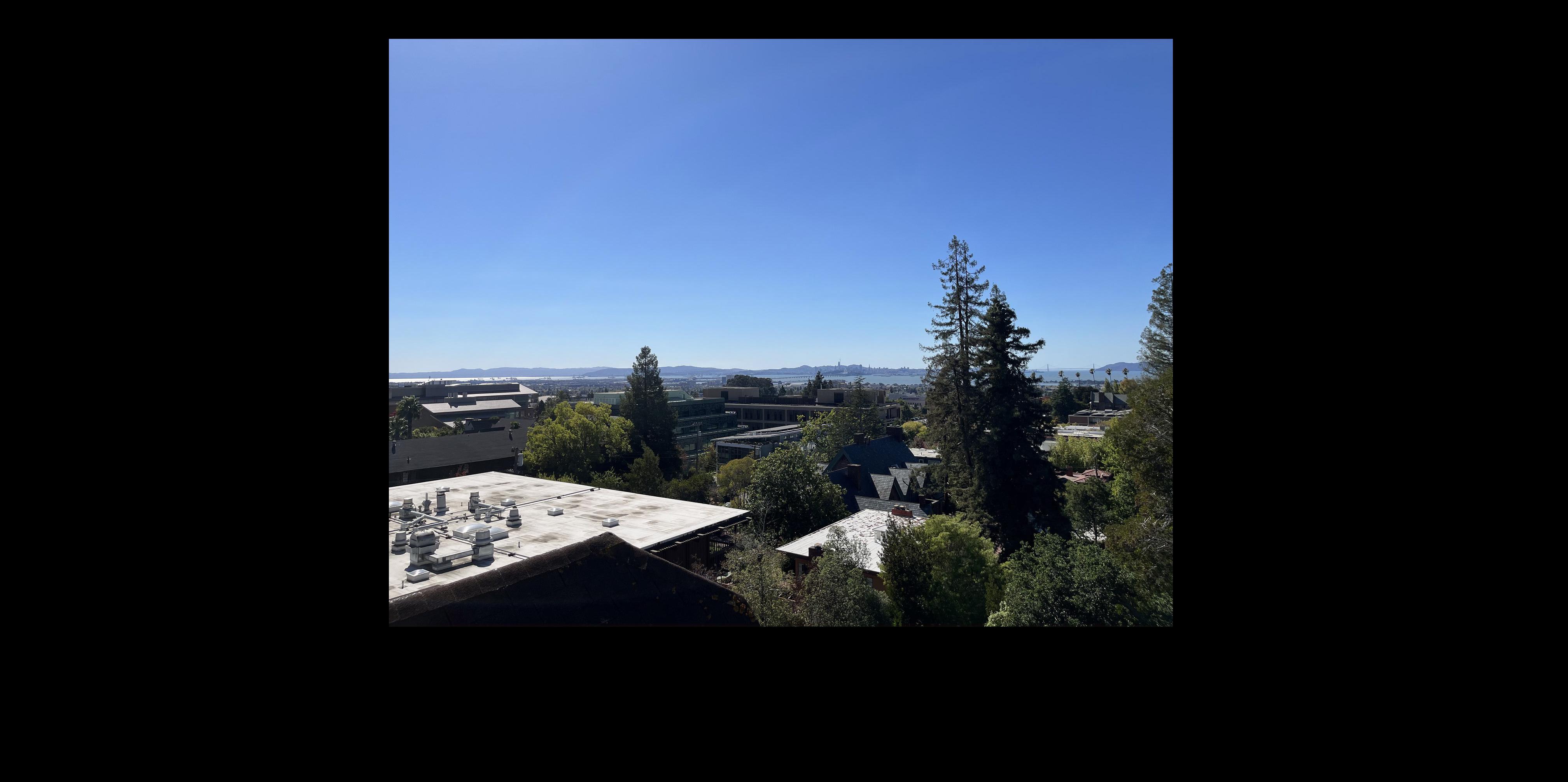
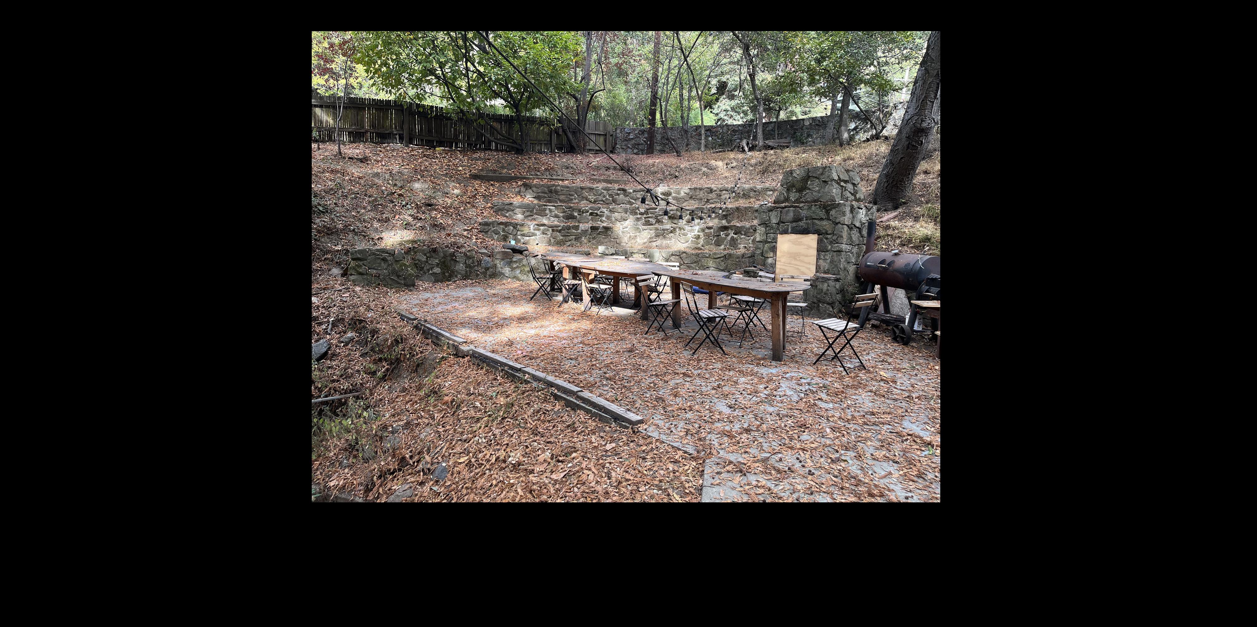
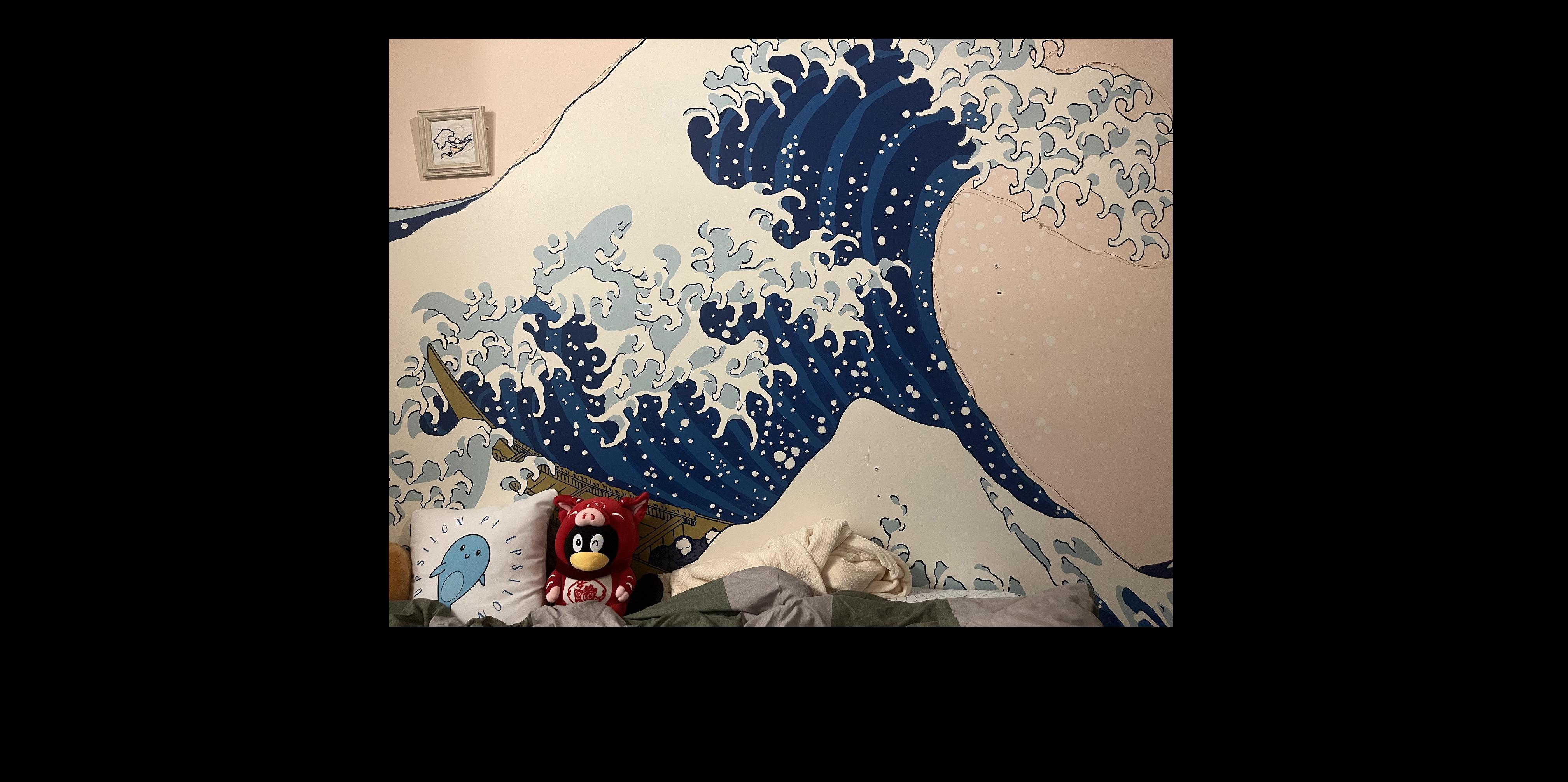
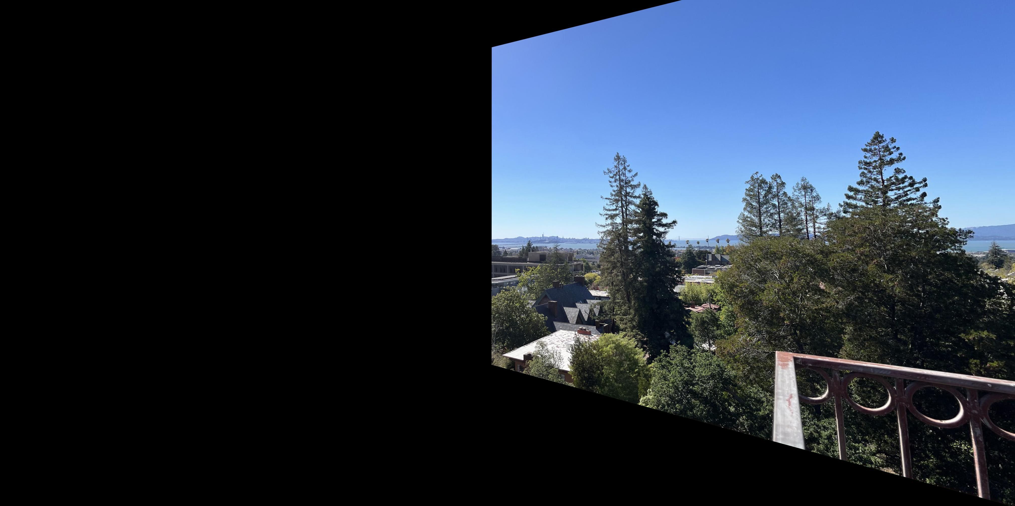
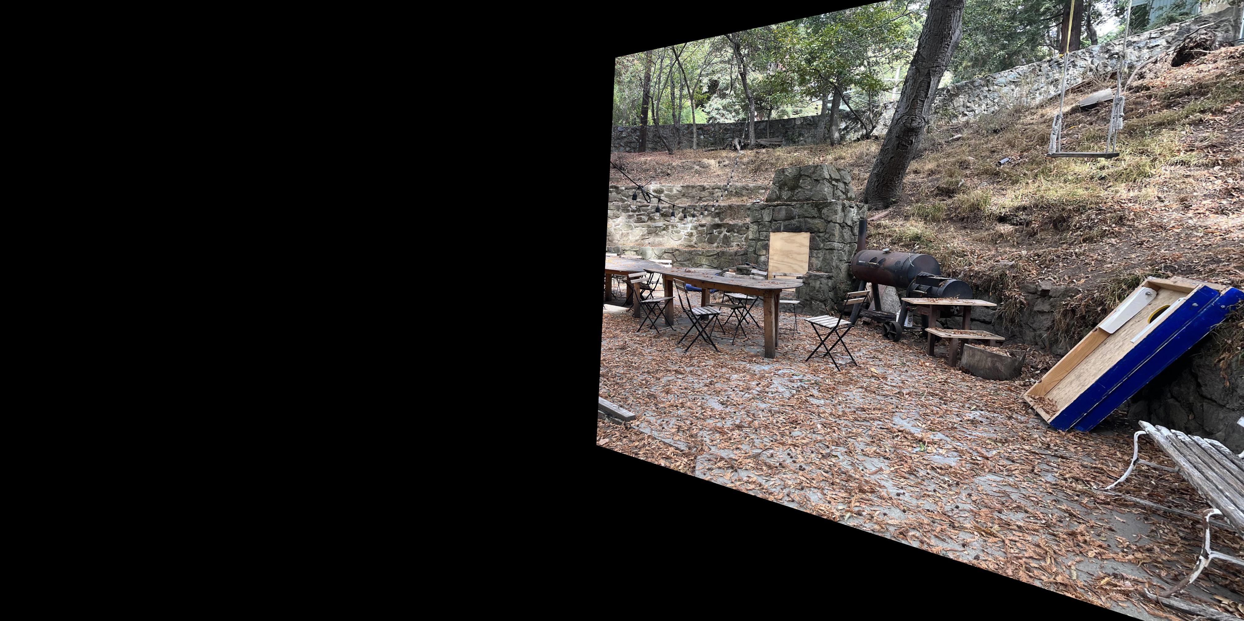
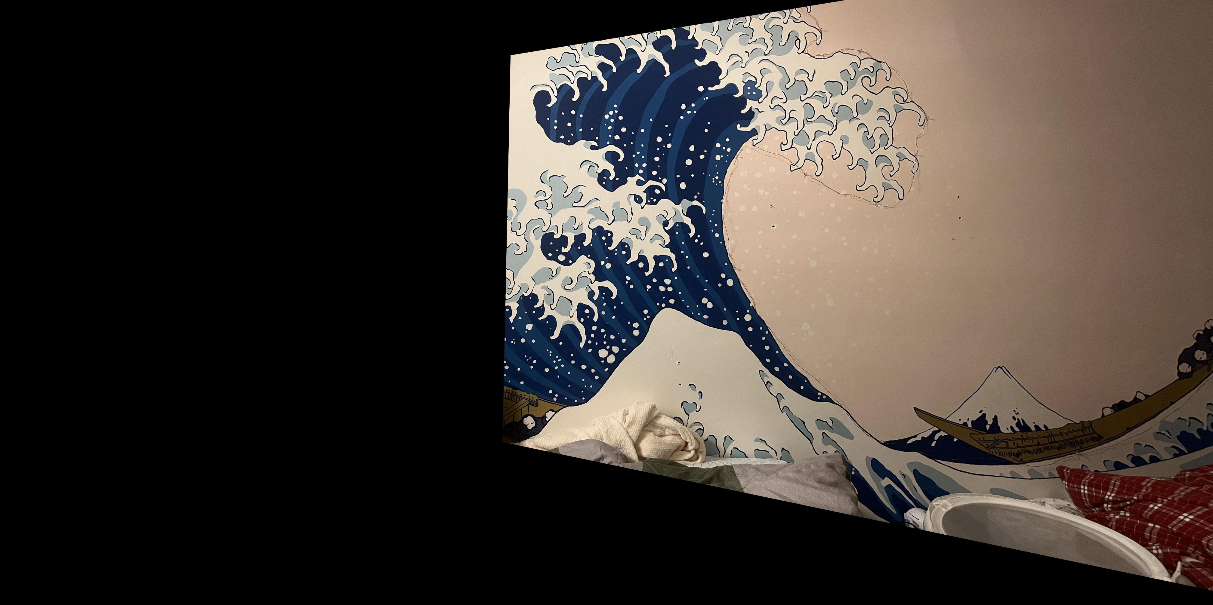
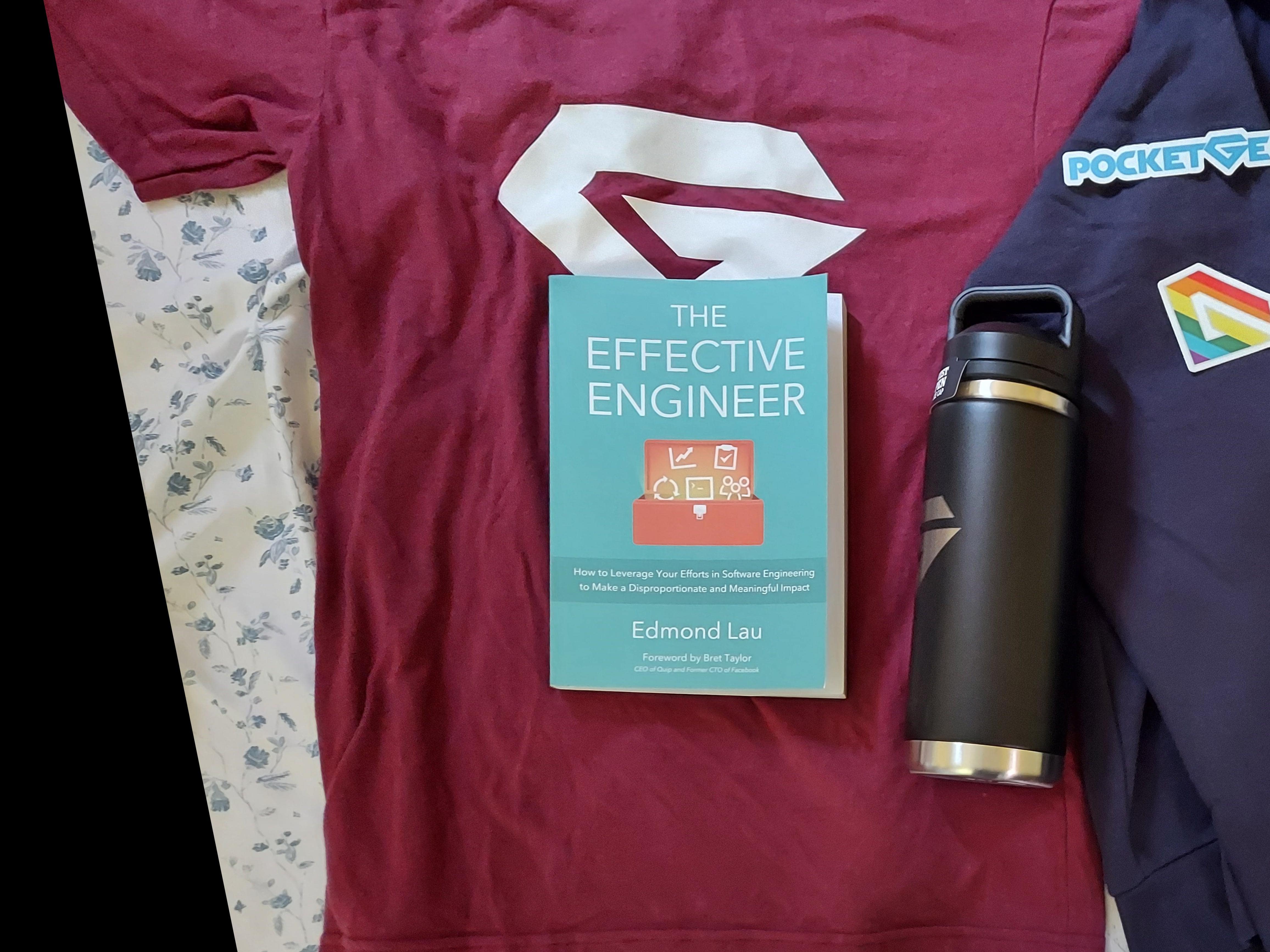
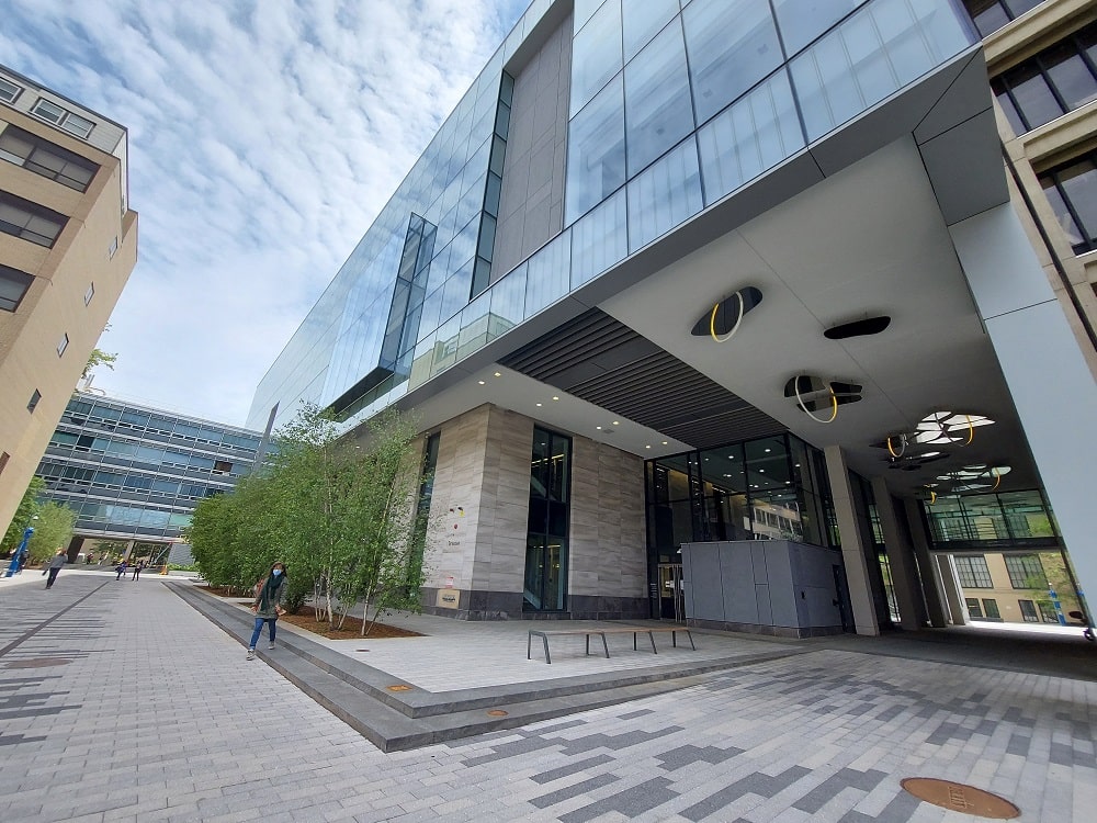
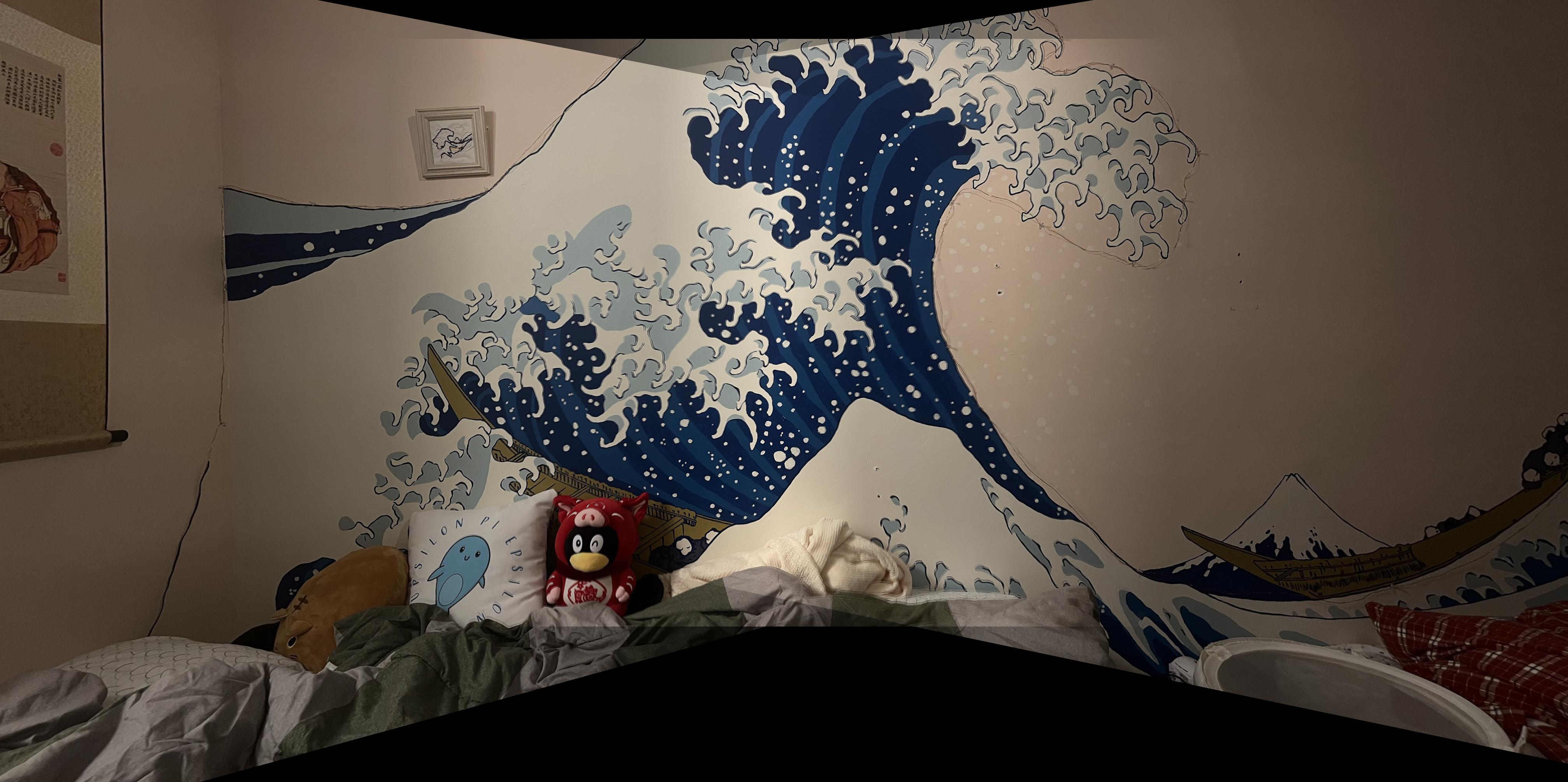
First, I shoot the pictures following the guidelines. I shot three sets. First a faraway scene(the scene on the top of my roof), then a medium-distanced scene(in my back yard), then a set of relatively close shots in dim lighting(in my bedroom at night). The original images are shown below.
Note: I forgot to turn on the AE/AF lock when taking the faraway scene picture. So the exposure were a bit different among the pictures.
Result Pictures
A-2 Recover Homographies
In this part, we manually selected corresponding keypoints between pictures, and then calculated homographies to project onw picture to the other using the formulas taught in class.
Algorithm Explain
First, we used plt.ginput similar to Project 2 and Project 3. I used 8 keypoints for each pair of pictures, and this value is set up as a variable that can be changed for later usages.
To warp an image from, say, projection defined by keypoint array arr2 to a new projection defined by keypoint array arr1, we first want to calculate the homography from the destination shape arr1 to the starting shape arr2 (note: because we are using inverse warping).
Specifically, to calculate the homography, we take the formula we have from class:
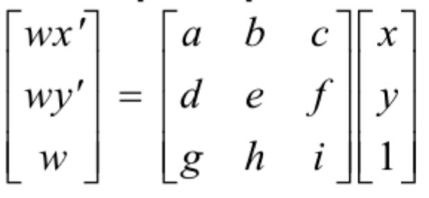
We can then break the matrix down, and stack the information from all n = 8 points together to form the new matrix function:
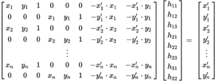
The above formula can be rewritten as A*h = b, while h can be rewritten as the 3x3 homography by copying the first 8 values in order and adding 1 as H3_3. So we can just construct A and b using the above formula and the keypoints we selected in the previous step, and use np.linalg.lstsq to calculate the H value.
A-3 Warp the Images
In this part, we warp the images to a certain position in a larger image that will form our final image
Algorithm explain
To warp the image, since we are using inverse warping, we need to apply the homography we calculated in previous part to points in the destination image, and then choose the best pixel value based on the value around the result point in the original source image. I used cv2.remap function here. For syntax and usage examples of this function, I referenced the documentation of this function: https://docs.opencv.org/3.0-beta/modules/imgproc/doc/geometric_transformations.html?highlight=remap#cv2.remap, as well as this thread: https://stackoverflow.com/questions/46520123/how-do-i-use-opencvs-remap-function. I did write all the code myself.
After warping the image to the new position, we can see below that the position of images are correct, but we would like the images to shift to the right a bit, since the images are larger after the projection transform, and we would like a larger image. As shown below, most of the leftmost image is actually cut off, and we don't want that.
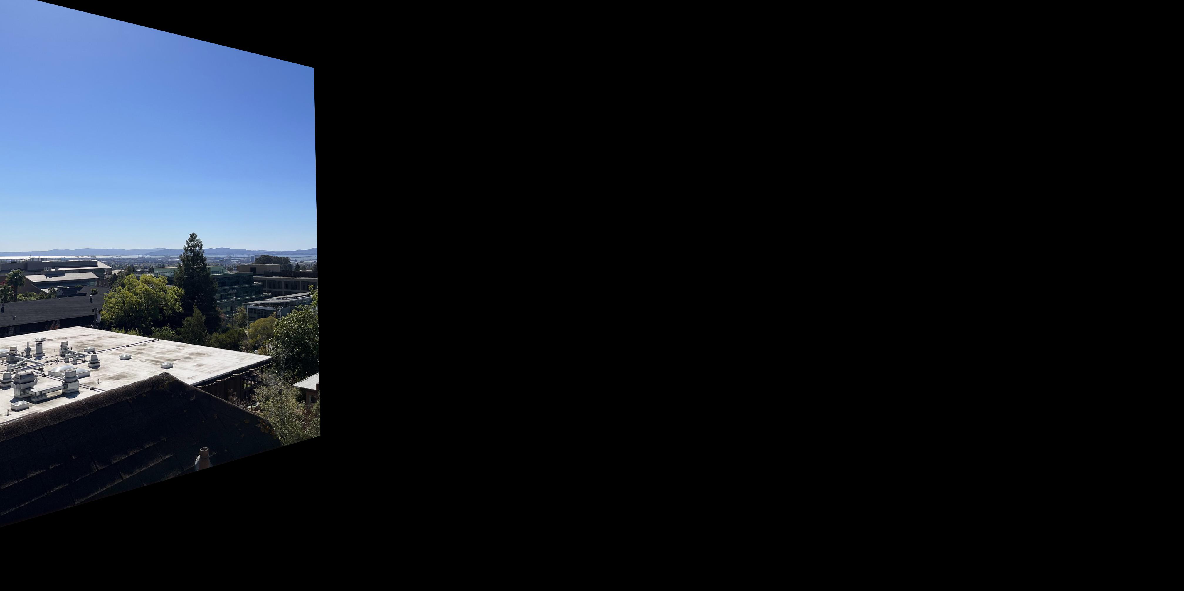
The solution is to add a dstSize and shift variables to the warpImage function. We make the result image dstSize so that we can fit all the stretched images in, and we can shift ALL the images by shift amount to fit them in the new window. To shift the image, we can just subtract the shift amount to all index_x and index_y elements.
The result look like following:
A-4 Image Rectification
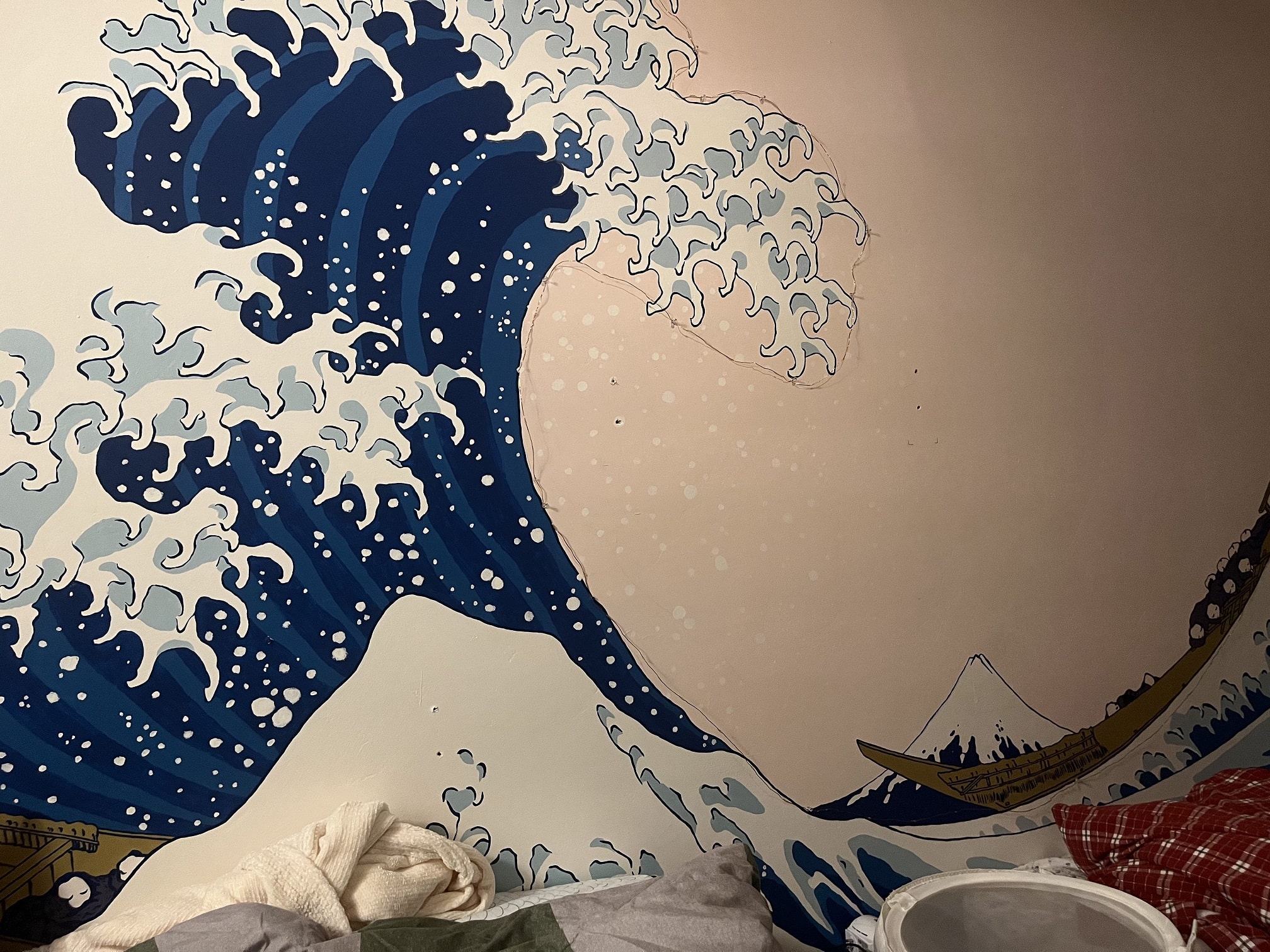
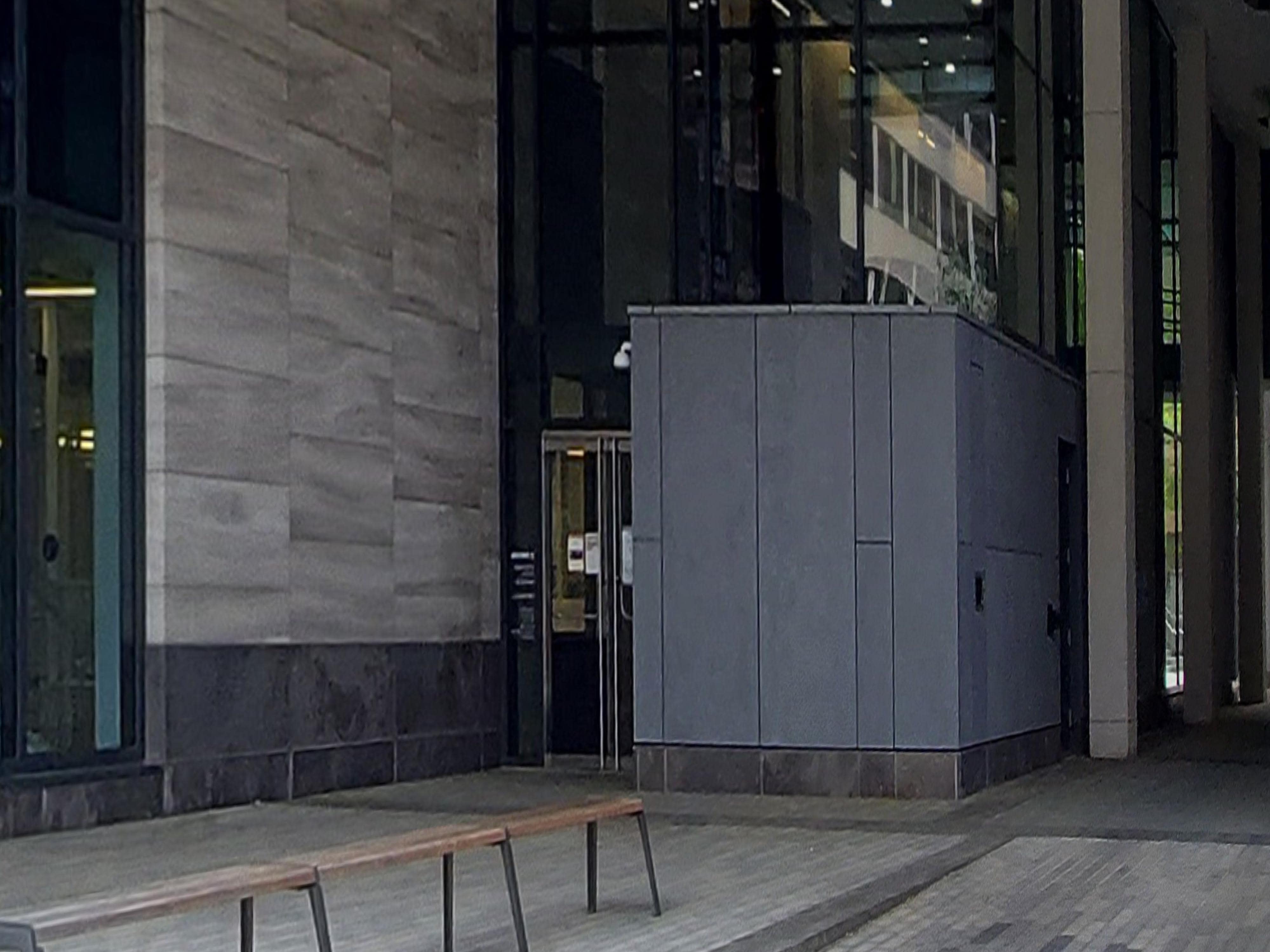
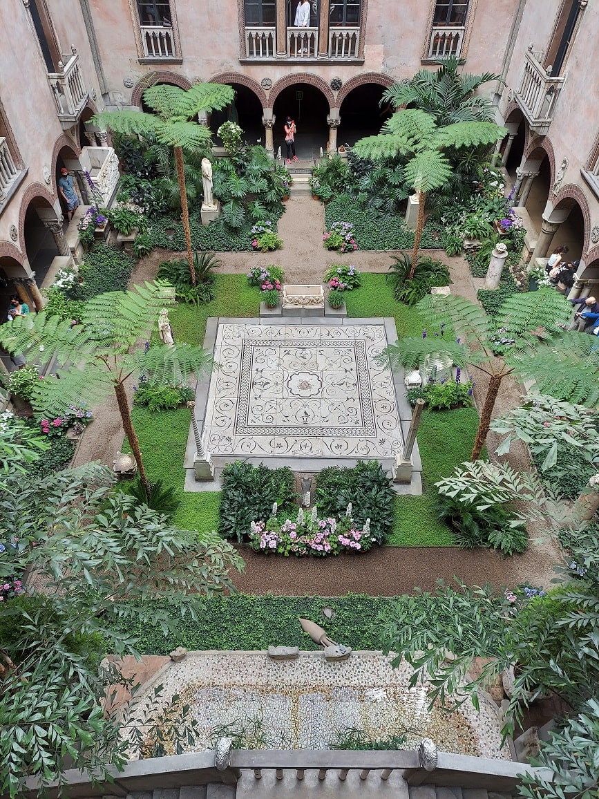
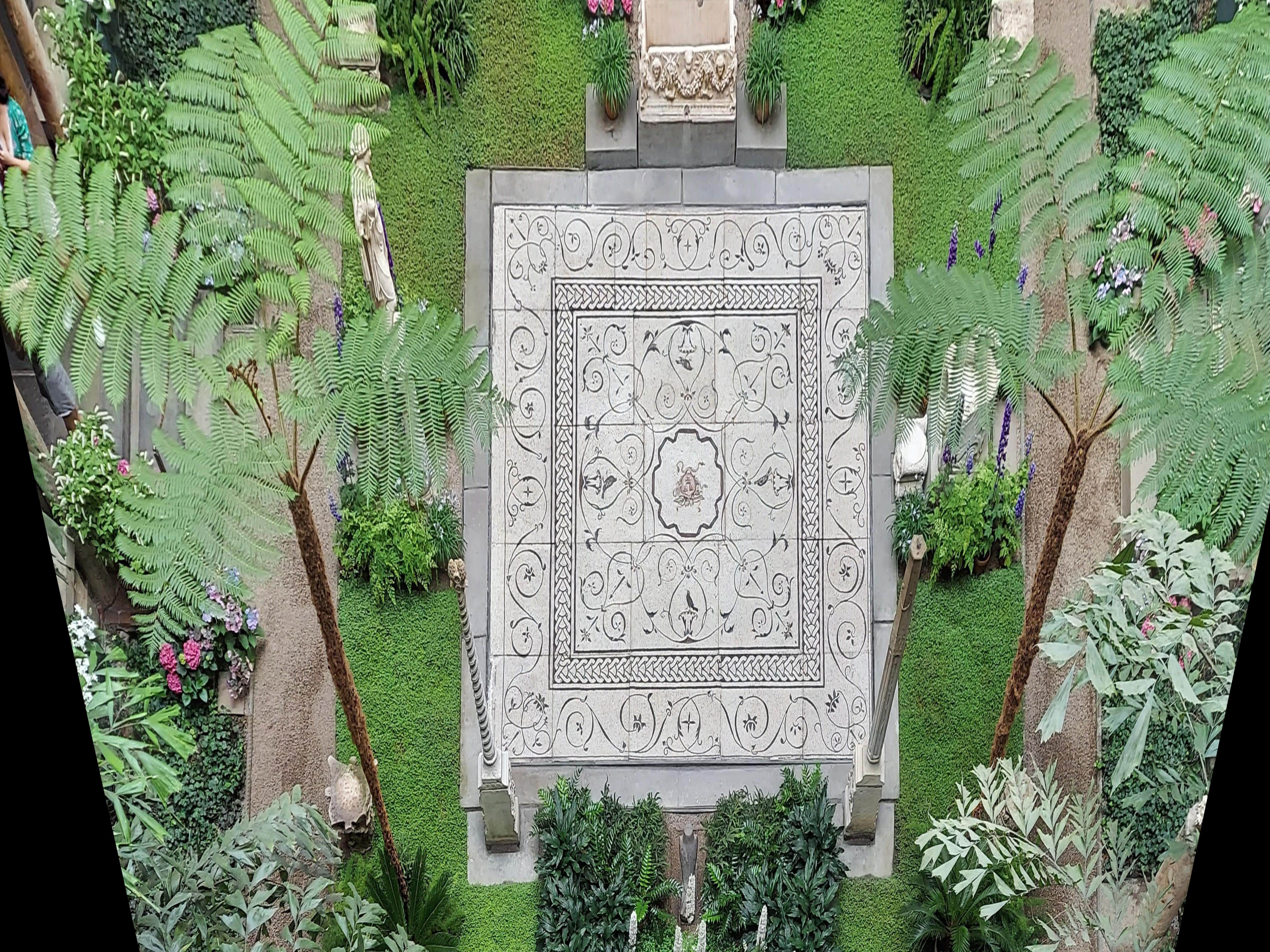
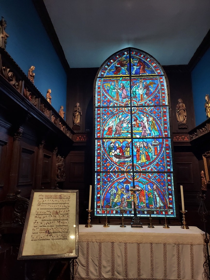
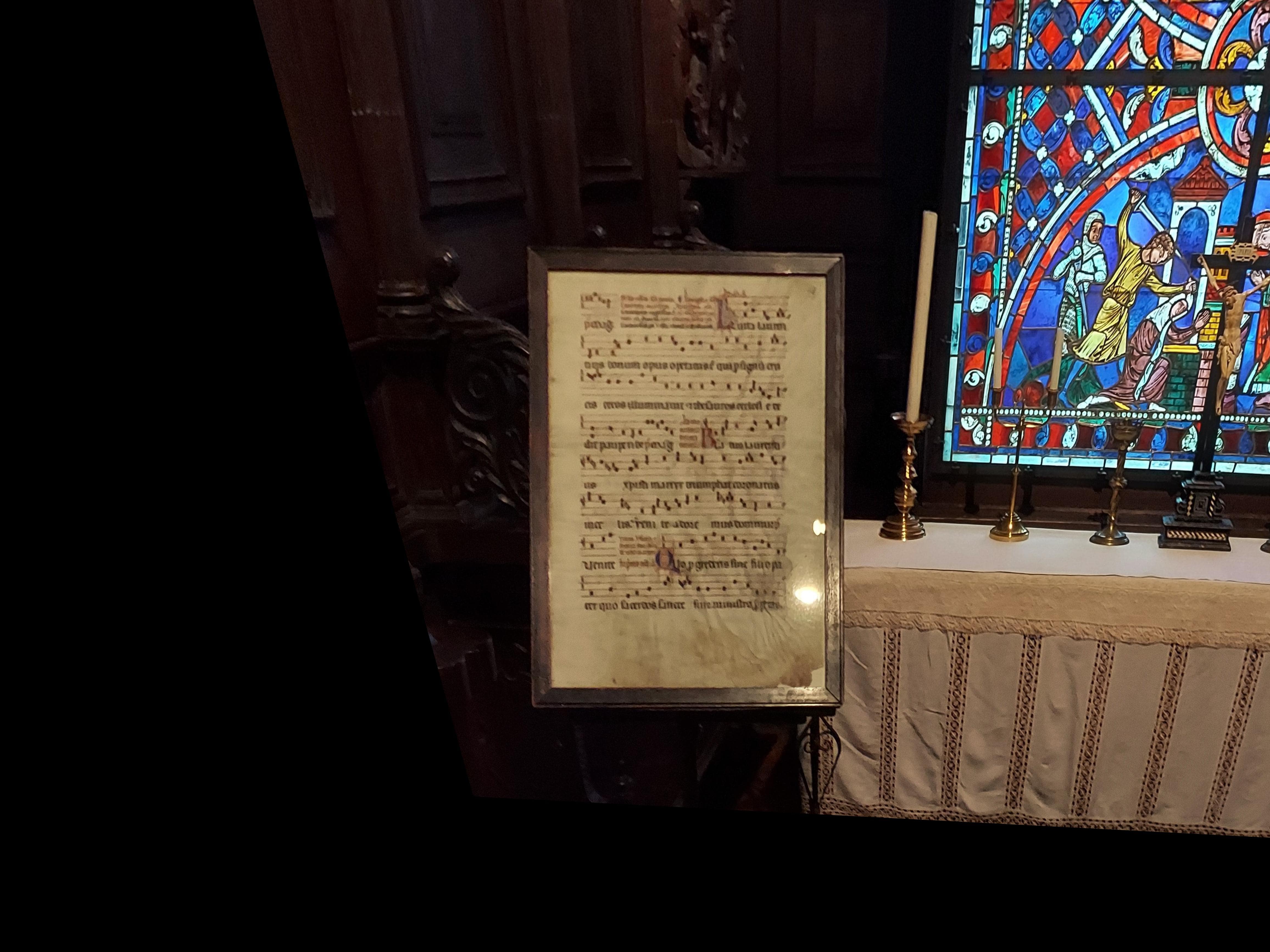
In this part, we try to "rectify" an image. Basically, we will wroite a program such that after choosing a plane in any image, we can use homography and warping to create a new image with that plane as frontal and in the middle, so that we can create the effect that we are looking at that surface directly from the front.
Original image and plane chosen:
A-5 Blend the images into a mosaic
In this part, I blended the warped images in previous parts together to form panoramas.
Algorithm Explain
As pointed out in lectures, simple piling up of the images could lead to an obvious edge in the panorama, which is obviously not ideal. I used a weighted average method using an alpha mask to achieve a smoother transition.
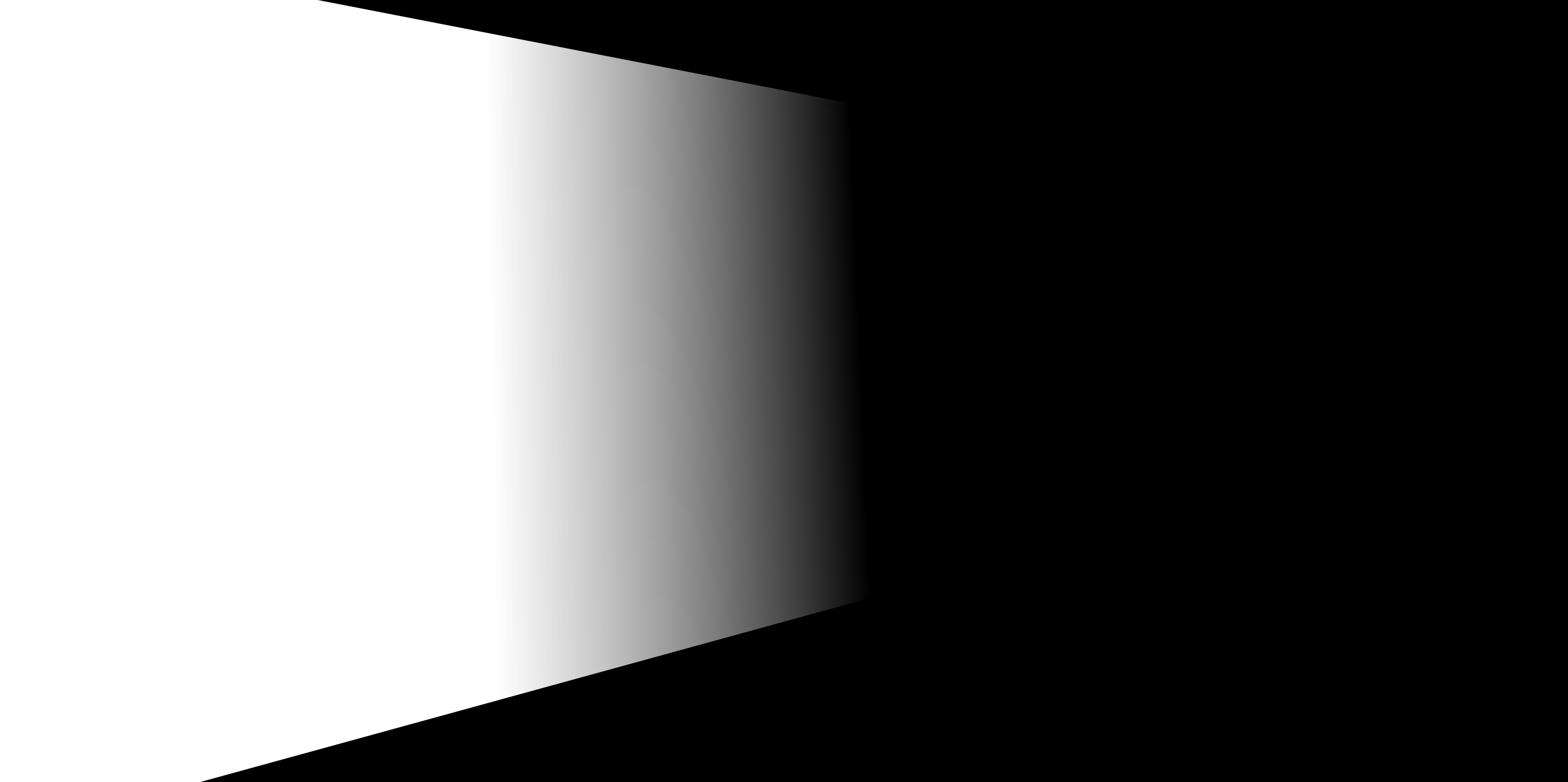
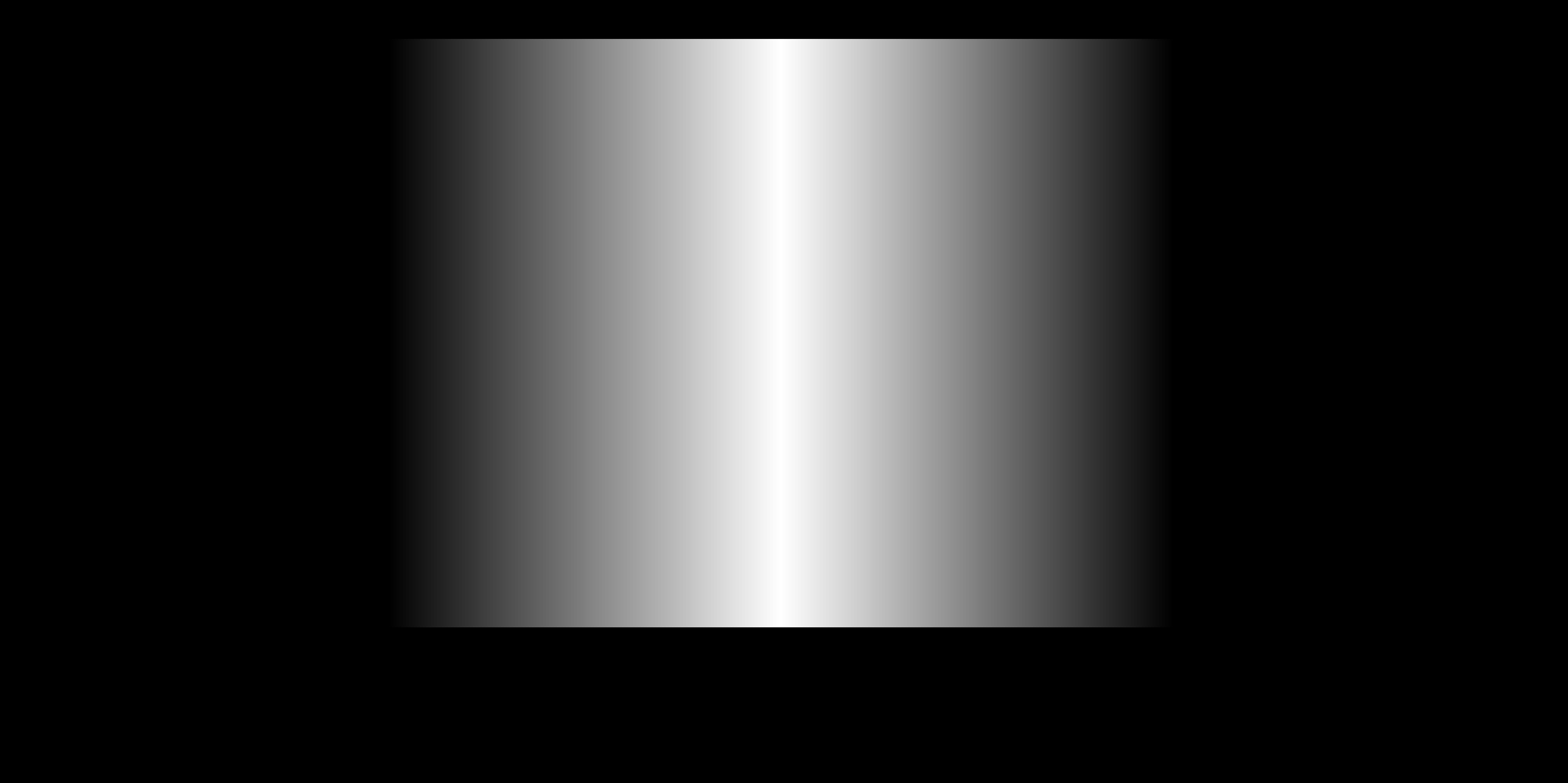
First, we make the three kinds of alpha mask in the original image space. I used np.linspace and np.tile functions to achieve linear fallback from the middle of the mask to the side of the mask.
In this part of the project, all the images I made are stiched together horizontally and span less than 180 degrees. So we only need 3 alpha mask. One for image on the left most, which only need fade out on the right side, One for the image on the right most, and one in the middle, with fade on both sides. The masks look like:


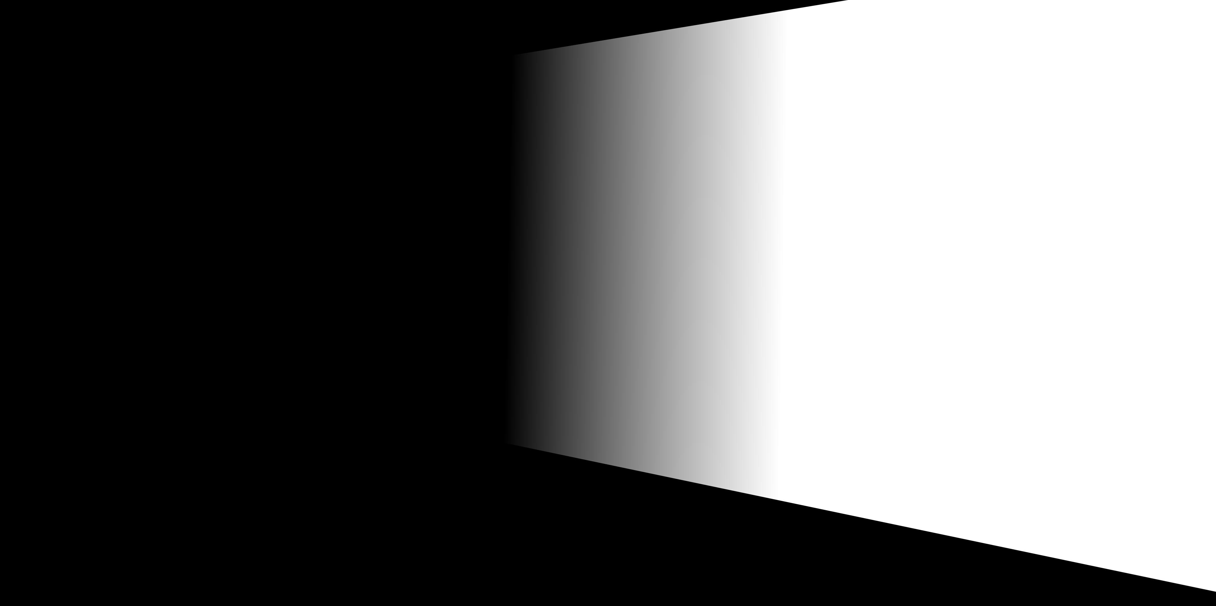
I then warped the masks using the same way we warped images in the previous part, and it looks like this. Note: we can also apply the mask and warp the images. But at this point I have the warped images already so I just went along with it.
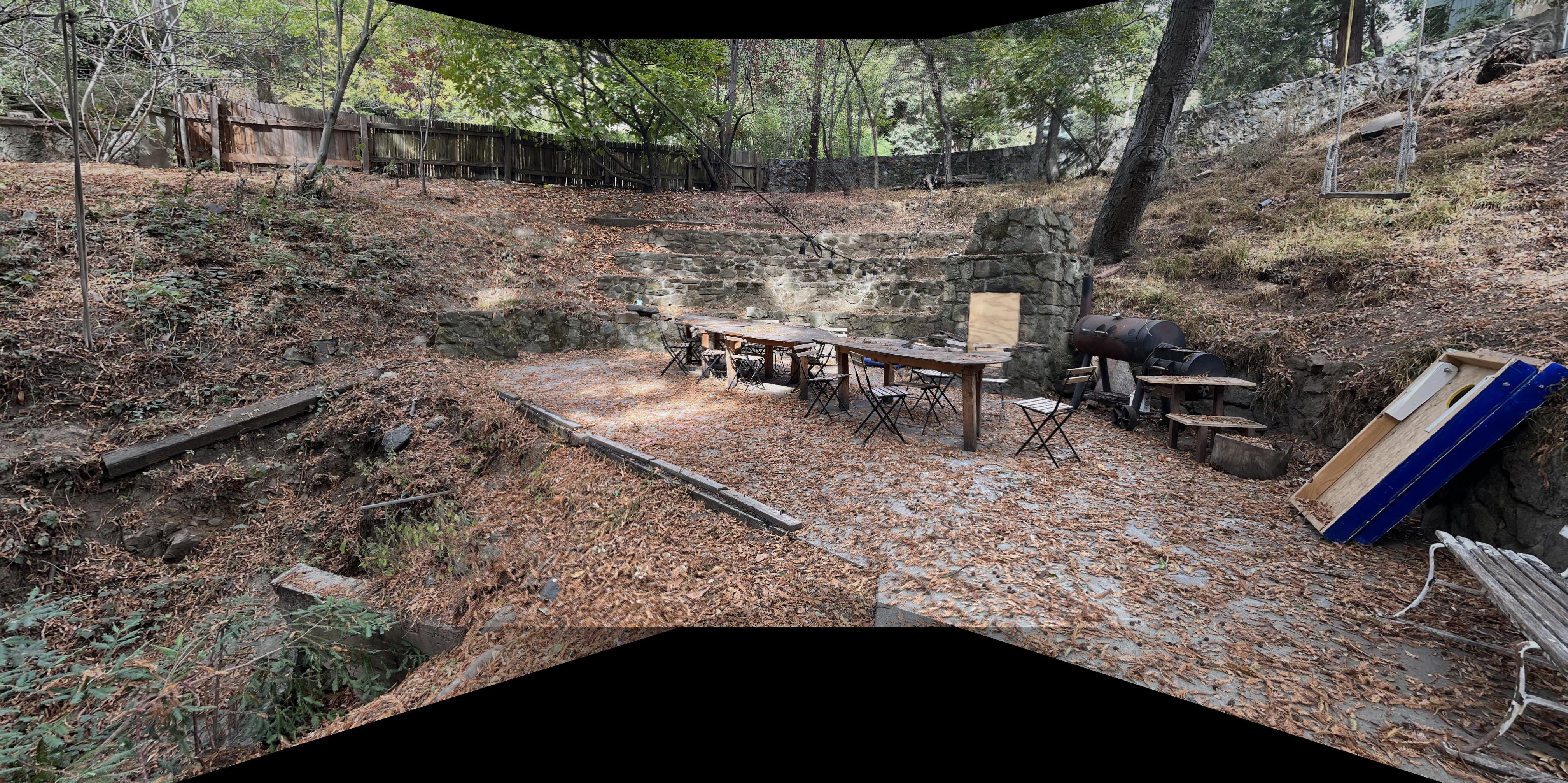
Last but definitely not least, we element-wise multiply each warped image to their corresponding warped alpha masks, and adding them together to form the final image! Results shown below:
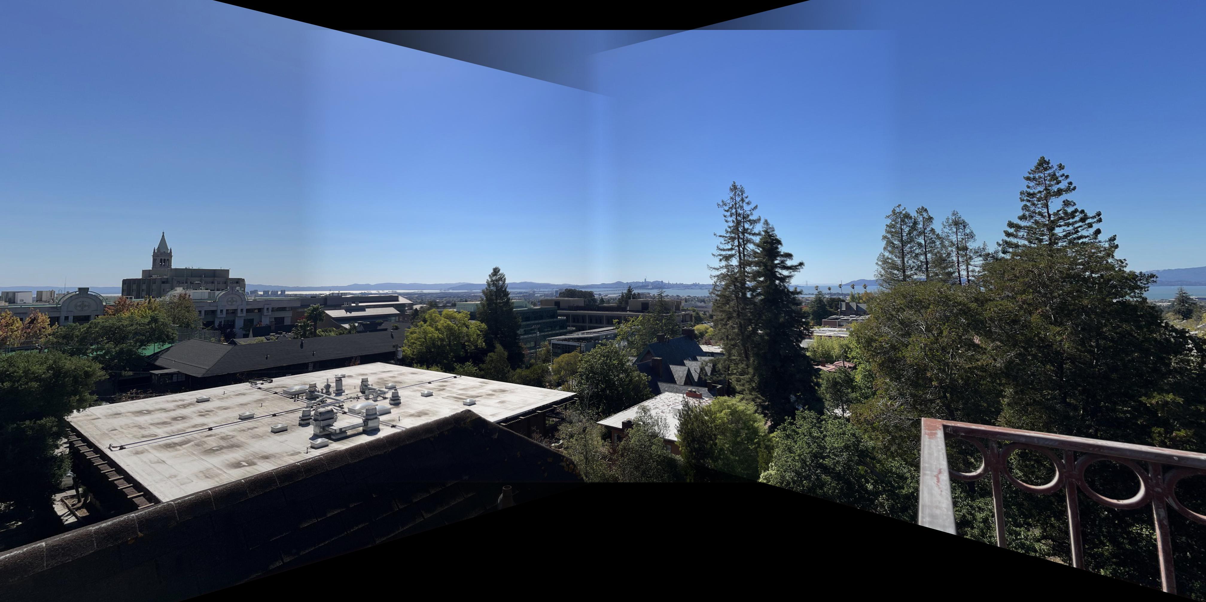
Note: In the first result, there were some inconsistencies. Since they don't appear in the second and third image, I think it is because I didn't lock the exposure when taking the first scene, causing different images to have inconsistent brightness. It could also be because of the blending method.
PartA: What I learned
In this part of the project, I learned how to calculate homography and how to warp images using the homography to a different projection. This is very exciting. I managed to produce ok looking panoramas with the relative naive solution: manual point selection, no calibration and alpha channel general blending. I hope to improve this in Part B, to make it automatic and robust against error. I am also VERY interested in taking 360 panoramas and form a cylinder or even a ball, and export it to view in Virtual Reality. I think it is going to be very cool and I hope I can finish that for Bells and Whistles.