Image mosaics & rectification

Last weekend, I went home to Sacramento. That means I took a train and enjoyed my surroundings as I traversed the 100 mile journey. Along the way, I snapped the following photos, and made mosaics out of them:

The view towards the train stairwell

The view towards the aisle

Well, before you see the results, let's explain how this works. I selected eight corresponding points on each image I took; each of those eight points represent the location of the same objects as they change position based on the rotation of the camera.
These corresponding points allow us to compute the homography of an image, which enables the transformations required for image stitching. In reality, just four points are required for homography, but additional points provide higher accuracy if well-placed.

I used the following matrix to estimate my homography matrices:

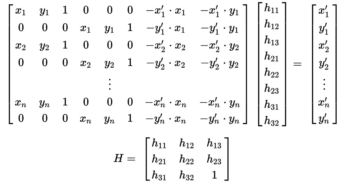
Then, plugging in the (x, y) pairs for each of my selected points below, I calculated the most likely entries of the 3x3 homography matrix via least squares.

Eight input points around rectangles in the train.

A mosaic of the two extends the view using just one image. As you can see, the rightmost photo is stretched such that its points align onto the left photo's points, which allows the two photos to extend each other.

A view of Scenic Blvd. going eastward to campus.

Going westward to downtown.

Eight input points around the sidewalk

A mosaic of the two.

Berkeley's train station with a train in-station!

Eight input points along the train.

A mosaic of the two.

Martinez's train station from my train.

Eight input points along the ouside of the station.

A mosaic of the two.

Rectification

Another possible application of homography is the extraction of non-square textures from the photo's environment into a square (or other shape of your choosing). By nature of matrix transformations, the opposite can also be done to project a texture onto some object in a photo.
In this case, I grabbed the train map from the wall and the textured sidewalk.

What's on that train poster?

Ah, yes, very clear.

Let's feel the bumps of the pedestrian crossing.

Ah, yes, so ADA-accessible.

Auto-stitching

Overall, the procedure to automatically stitch two images is as follows:

Retrieve the Harris corners

Harris points on the left side.

Harris points on the right side.

Harris corners are used as identifiers for features of images, and we'll use them to match our images' features. Running harris.py::harris_corners on my image outputs every Harris corner over five pixels from any image border.
However, there are a lot - perhaps not too many to be impossible to match and compute, but certainly enough to make waiting for it excruciatingly painful.
Additionally, not all features appear on both images, so not every Harris corner can correspond to another.

Suppress points

Harris points on the left side.

After point suppression

To reduce the number of points in the image, single out the "strongest" corner in a given radius around each point, and eliminate the rest.
If this process doesn't remove enough points, just do it again more powerfully!
I implemented ANMS as outlined in the paper, starting by scanning within a distance of 10 pixels around any given point; as I removed more points I added an additional 4 pixels to this distance.
Then, I ran point suppression until I reached 850 points. For a 1200x900 image, I'd usually start with over 4000 points, so I'd usually narrow down to just one in five.

Match feature descriptors

(Zoomed out 80x80 patch for context)

40x40 local patch

Gaussian blurred down to 8x8

For each corner point, extract an 8x8 patch around it, sampled from a 40x40 Gaussian blurred window around that corner. The patches have their mean subtracted and standard deviation divided from them for normalization.
The, match points by comparing their respective feature descriptors using SSD.
A correspondence is defined between two points if the ratio of the SSD error for the two descriptors and the SSD between the descriptor for the second-best match is less than 0.15;
that means that there's one particularly clear match for a descriptor, rather than two or more that are indistinguishable.

RANSAC

The matched patches, numbered.

The autostitched result

The manually stitched version

After retrieving a set of at least four matches, we can compute a homography matrix. However, to eliminate the effect of mismatches and outliers, the RANSAC algorithm comes in handy.
For each of 1200 iterations, 4 random points are sampled as inputs, and the number of matched features between the two images informs which homography matrix is best suited towards the final autostitching.
After recomputing a final least squares homography matrix between all of the >4 matched features, the images are stitched together.

Results

The matched patches, numbered.

Martinez autostitched

Martinez manually stitched

The matched patches, numbered.

Scenic Boulevard autostitched

Scenic Boulevard manually stitched

The matched patches, numbered.

The Carquinez bridge

Lots of great corners on the train!

Looks like I took a wrong turn. Anyone know how to get from "Benley" to Berkeley?

(autostitched)

Berkeley's station manually stitched

The matched patches, numbered.

The sky above my house.

Learnings

On the whole, the autostitching does a good, but not perfect job. There are some points where the autostitch clearly misses on the edges, like when the Berkeley sign instead read "BENLEY" above. However, in most cases, it came very close to my hand-selected points based matching, and most features on the edges are off by only a few pixels at most.

If there's one thing I learned from this project, it's that you should never flip your X and Y indices. It takes hours of debugging to fix related issues.

In terms of photography, camera settings matter a lot, and my phone is constantly changing settings to make sure that the entire pixel space is being taken up. However, it's in scenarios like stitching where these factors need to be held constant, as many of my photos have obvious changes in the color of the sky change.

Finally, I learned that a little statistics and random sampling can go a long way for making practical algorithms, even if it technically isn't deterministic. In this case, RANSAC almost always returned the same number of points each time it was run.

Morphing

Homography

Shooting pictures

Rectification

Auto-stitching

Retrieve the Harris corners

Suppress points

Match feature descriptors

RANSAC

Results

Learnings