Project 4: Image Warping and Mosaic
Aaron Sun 3033976755 Fall 2021
Shoot the Pictures
First we took photos which we would later rectify. This means we took photos of planes from a certain perspective, so that we could eventually warp them such that the scene was front parallel.
Then we took images which we intended to combine into mosaics:
Recover Homographies
Our problem statement is given as recovering a 3x3 matrix H = [[a, b, c], [d, e, f], [g, h, 1]] such that Hz_1 = z_2 for our set of corresponding points. When we write out the equations, we find that for a given correspondence z1 = (x1, y1) and z2 = (x2, y2):
x2 * w2 = a*x1 + b*y1 + c
y2 * w2 = d*x1 + e*y1 + f
w2 = g*x1 + h*y1 + 1
We can combine and rearrange these equations:
-x2 = -a * x1 - b * y1 - c + g * x1 * x2 + h * y1 * x2
-y2 = -d * x1 - e * y1 - f + g * x1 * y2 + h * y1 * y2
Finally we can make this a least squares problem Ax = b for x = [a, b, c, d, e, f, g]^T where each correspondence contribues in A the rows:
[[-x1, -y1, -1, 0, 0, 0, x1 * x2, y1 * x2], [0, 0, 0, -x1, -y1, -1, x2 * y2, y1 * y2]]
and these match rows in b:
[[-x2], [-y2]].
Warp the Images
Then we warped the images using the homographies we recovered. To do this, we took the homography and applied it to the 4 corners of the input image. Then we ued the inverse of the homography to find where in the original image each pixel in the output mapped to. Finally using bilinear interpolation we found the values of each pixel.
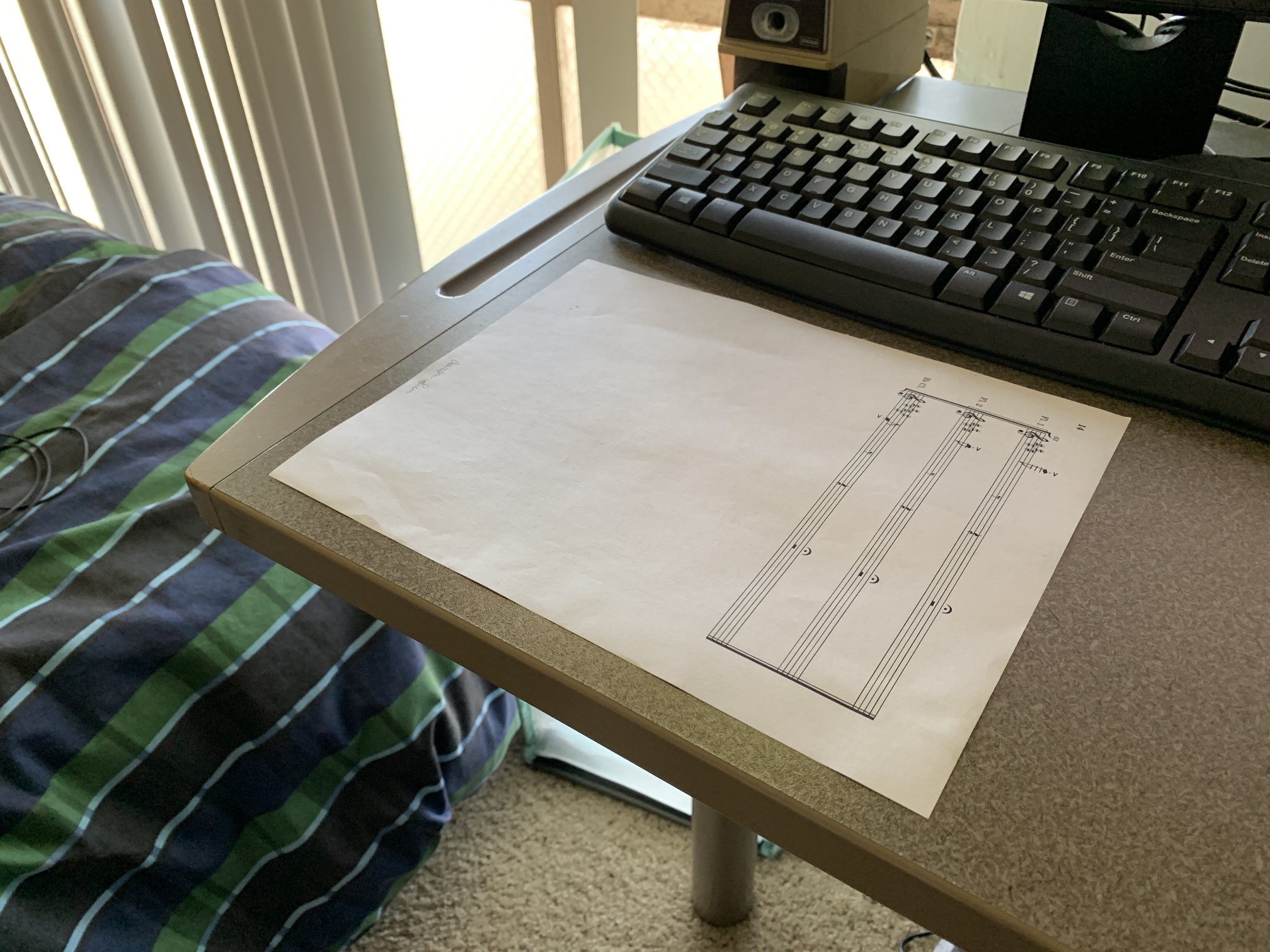
Let's look at our results for rectifying images. First, let's look at the sheet of paper on the table.
We mapped the corners of the piece of paper to the points [0, 0], [11, 0], [11, 8.5], [0, 8.5] (scaled by a fixed constant). This is making use of the fact that we know the actual size of the paper. The output paper comes out very nicely. Let's look at it a bit more closely:
Wow it looks great! We can even read the notes as if we were looking straight at the page.
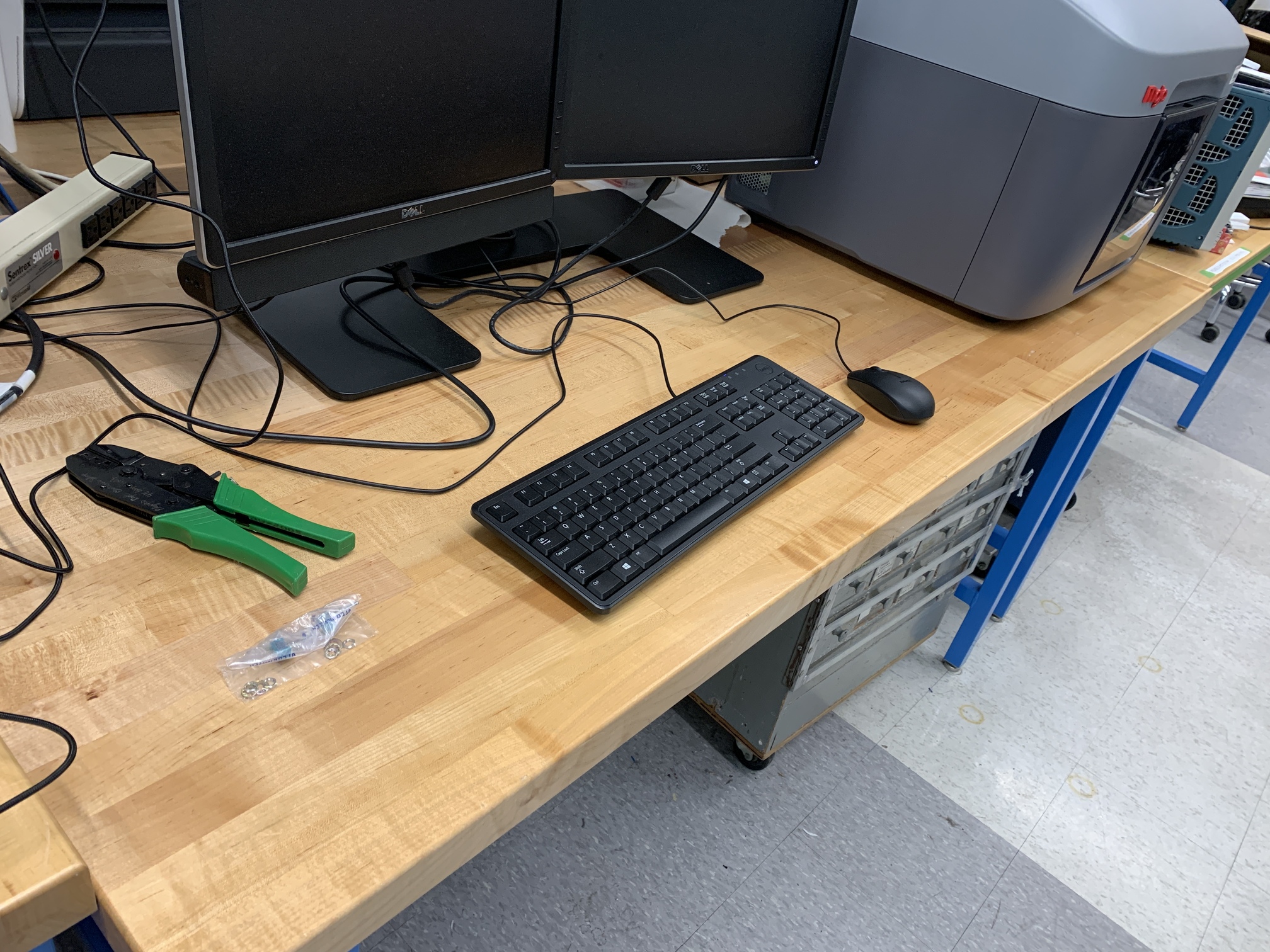
Let's try the same thing with the keyboard. I estimated the keyboard to have a width to height ratio of 10:3.
And now looking more closely at the keyboard itself:
Blending the Images into a Mosaic
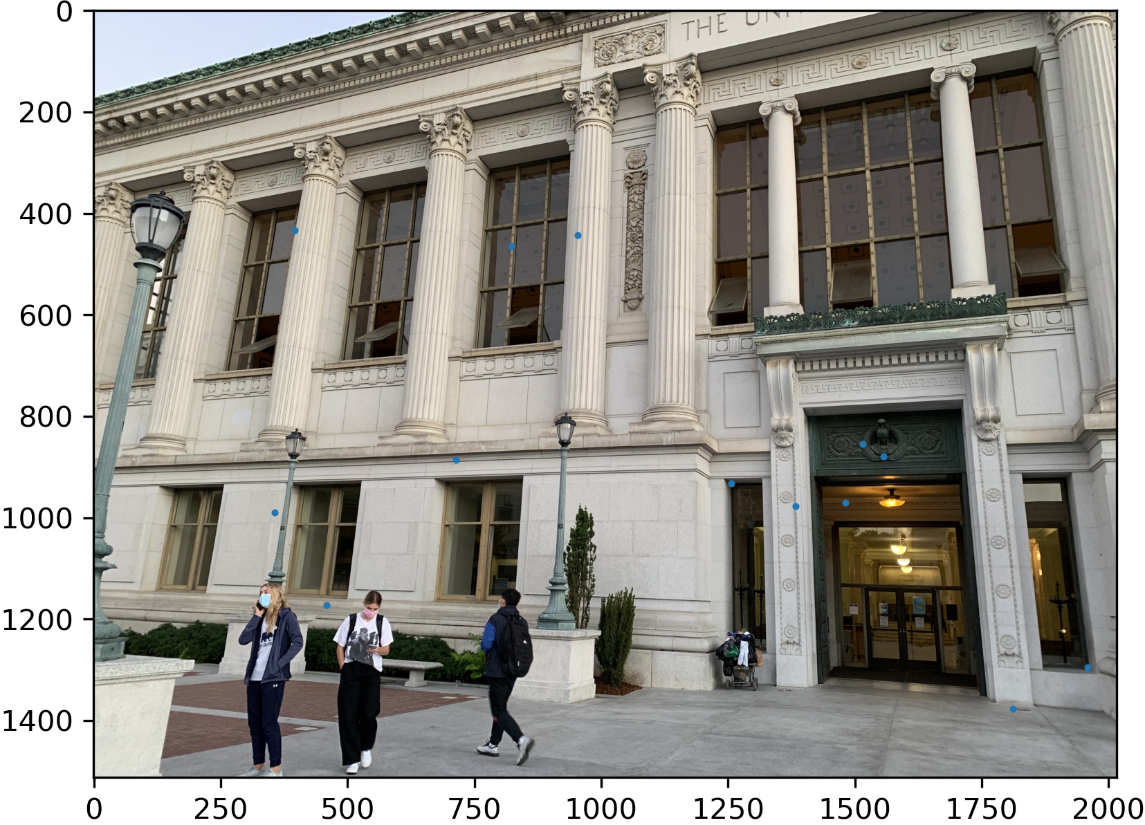
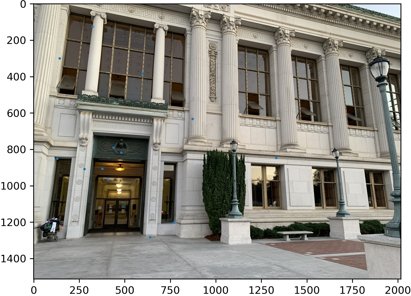
Now we can pick points as correspondences between our images and combine them into mosaics.
We first find the homography H to map image 1 to image 2. Then once image 1 is in "image 2 space" we combine the images. The combining process involves using the blending procedure from project 2.
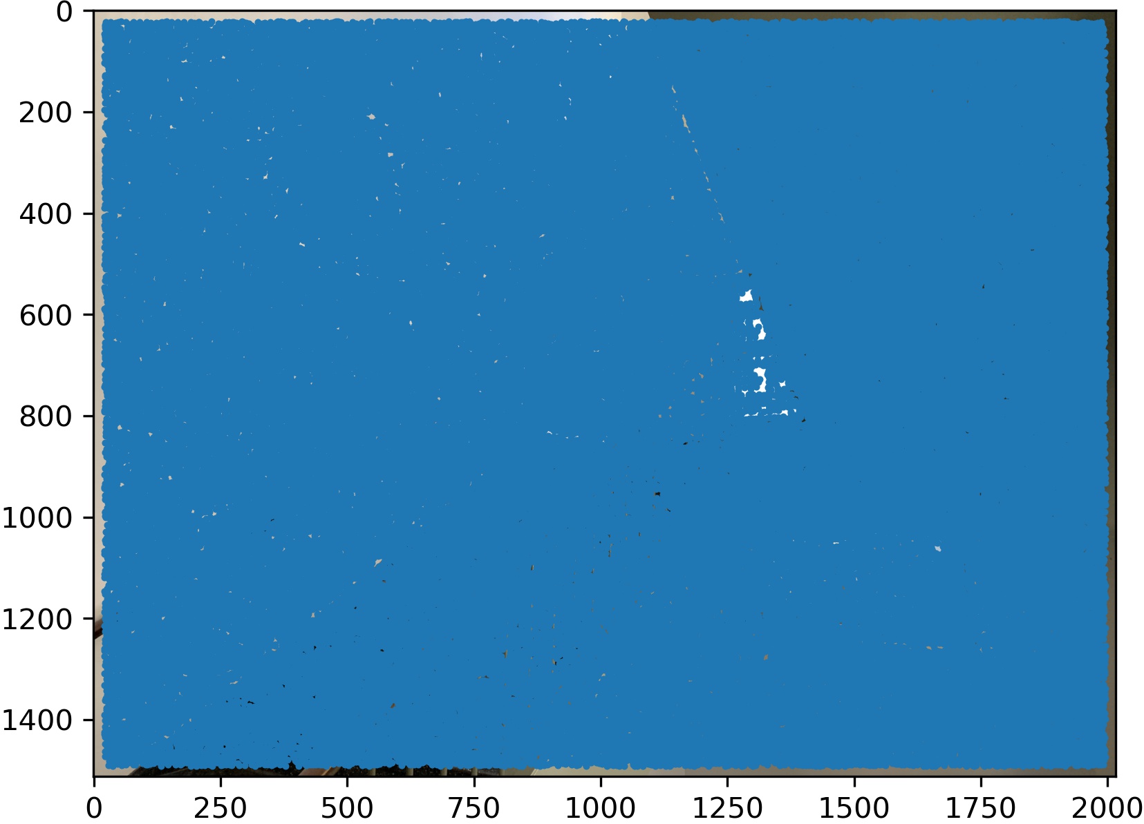
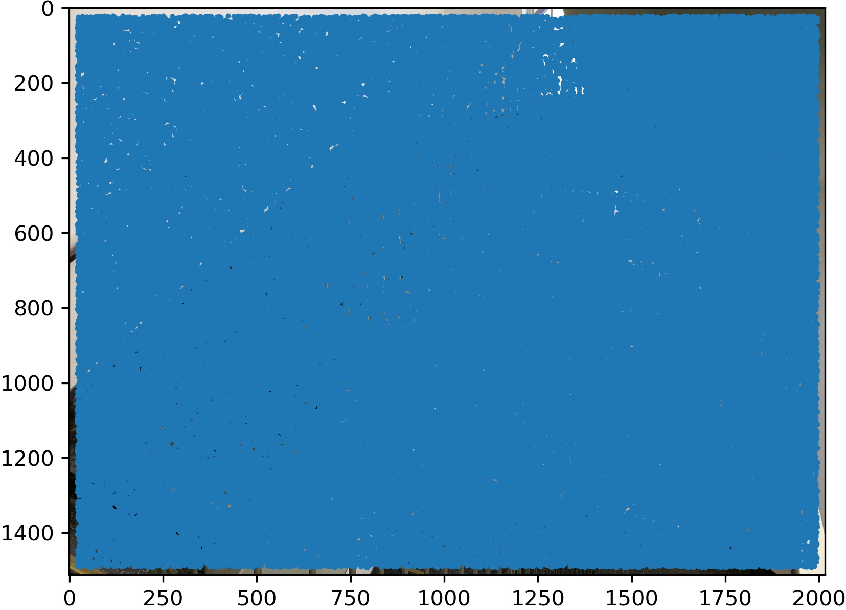
Choosing a mask automatically was a bit more tricky. First, we set a mask of all zeros. Then, we set pixels in which image 1 is nonzero but image 2 is zero to be 1.
We want the mask to be in the overlap between the images for good blending, so we need to extend the mask. To do this, we repeatedly dilate the image using a 3x3 convolution. We repeat this 20 times.
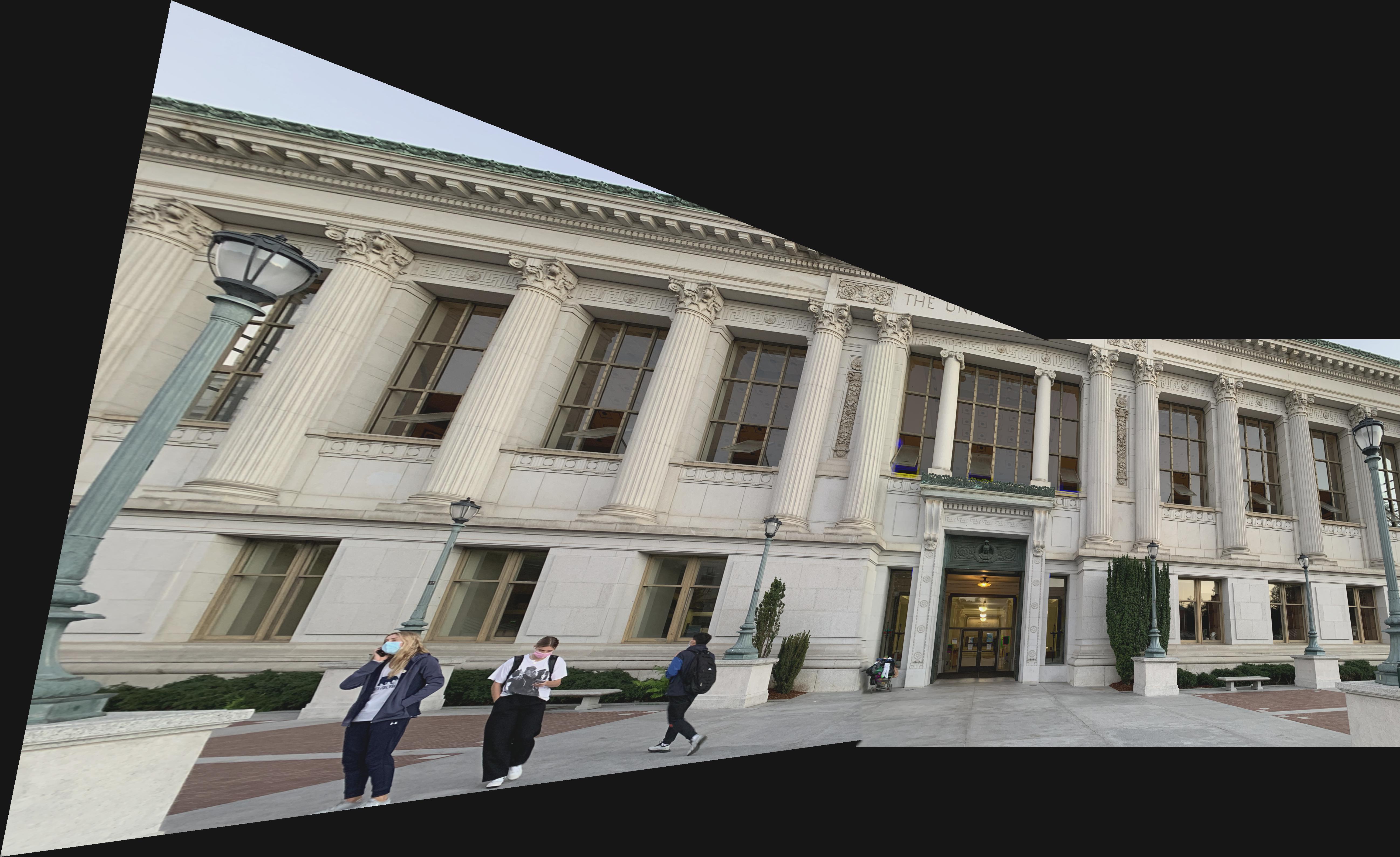
Then we blend the image as in project 2. Notably we used sigma = 3 and a pyramid of height = 2 in order to save time. This gives us the resulting images we desire.
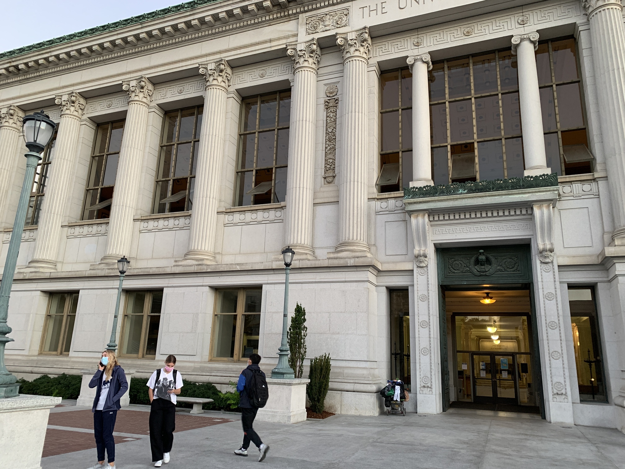
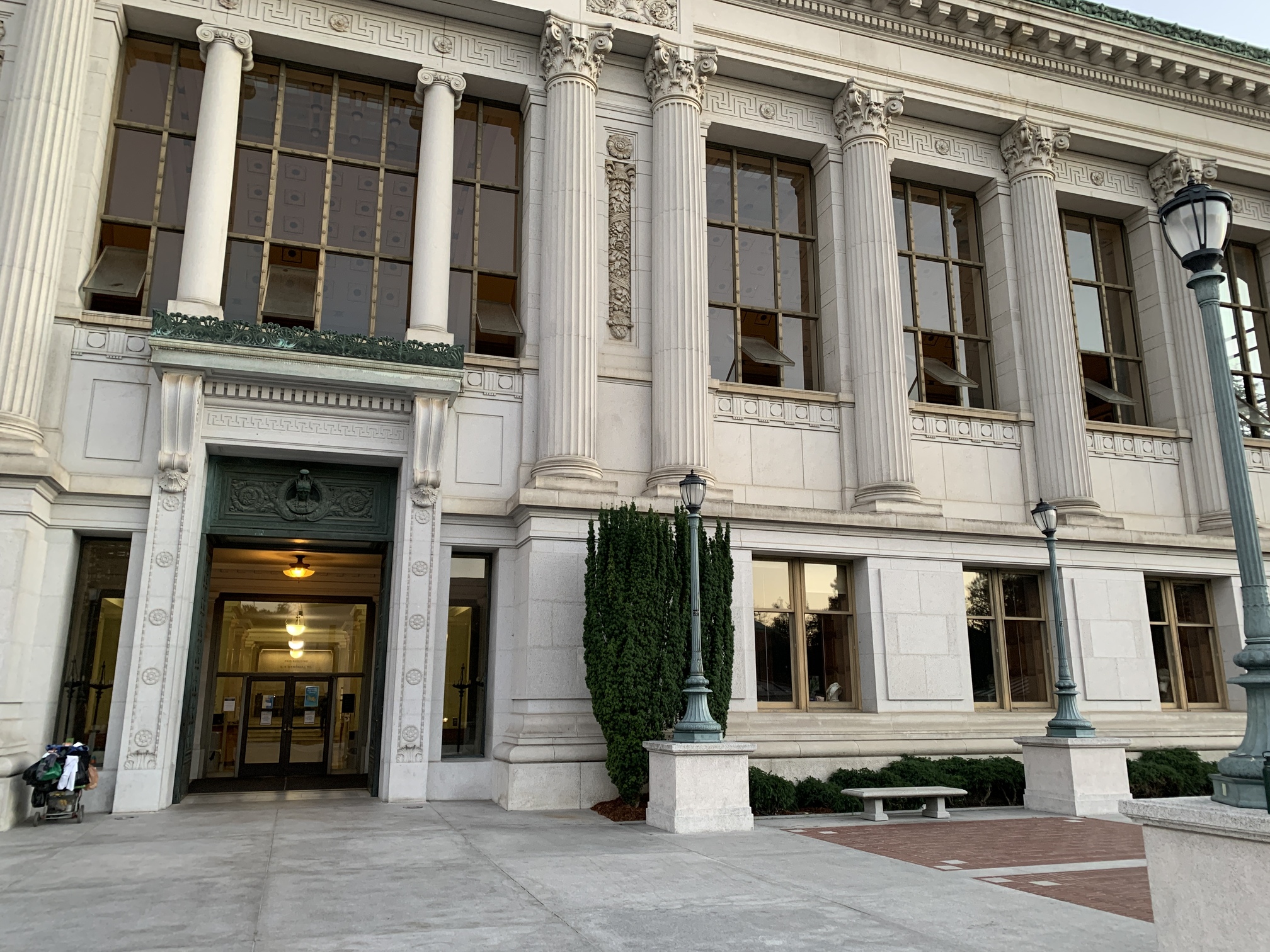
Doe library, in a wide view:
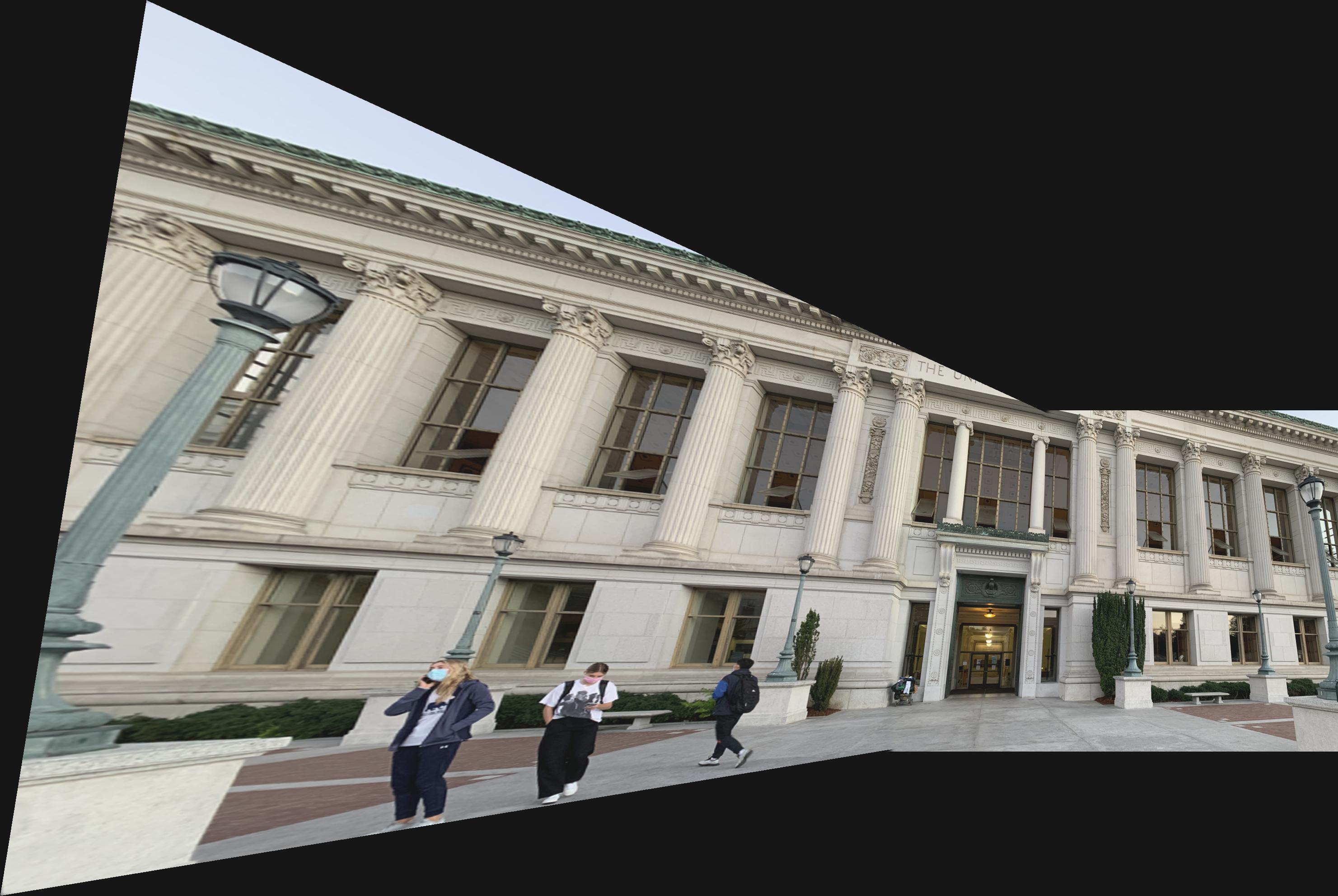
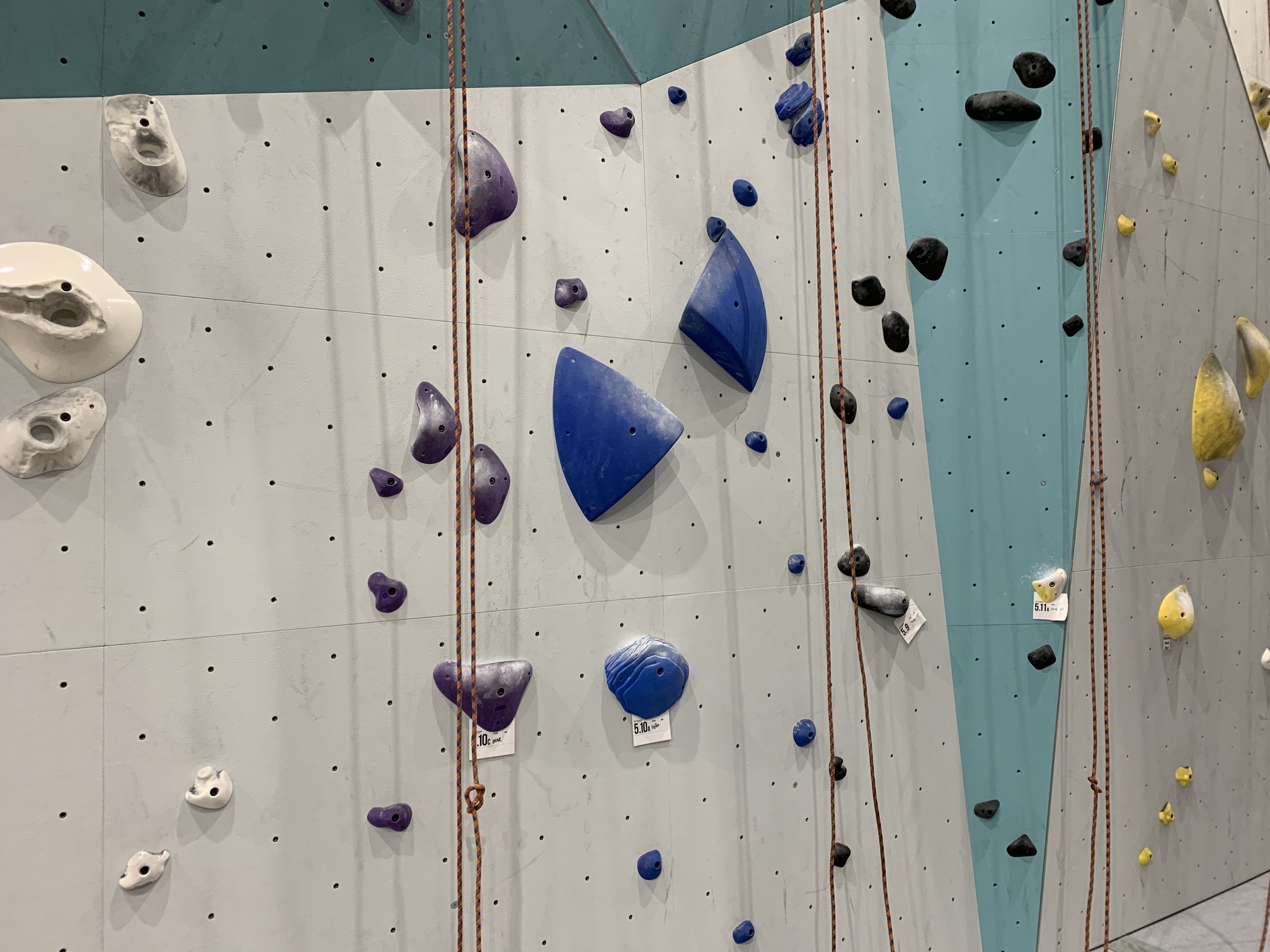
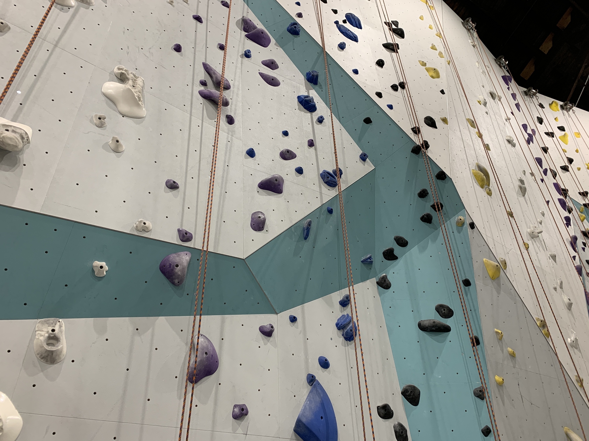
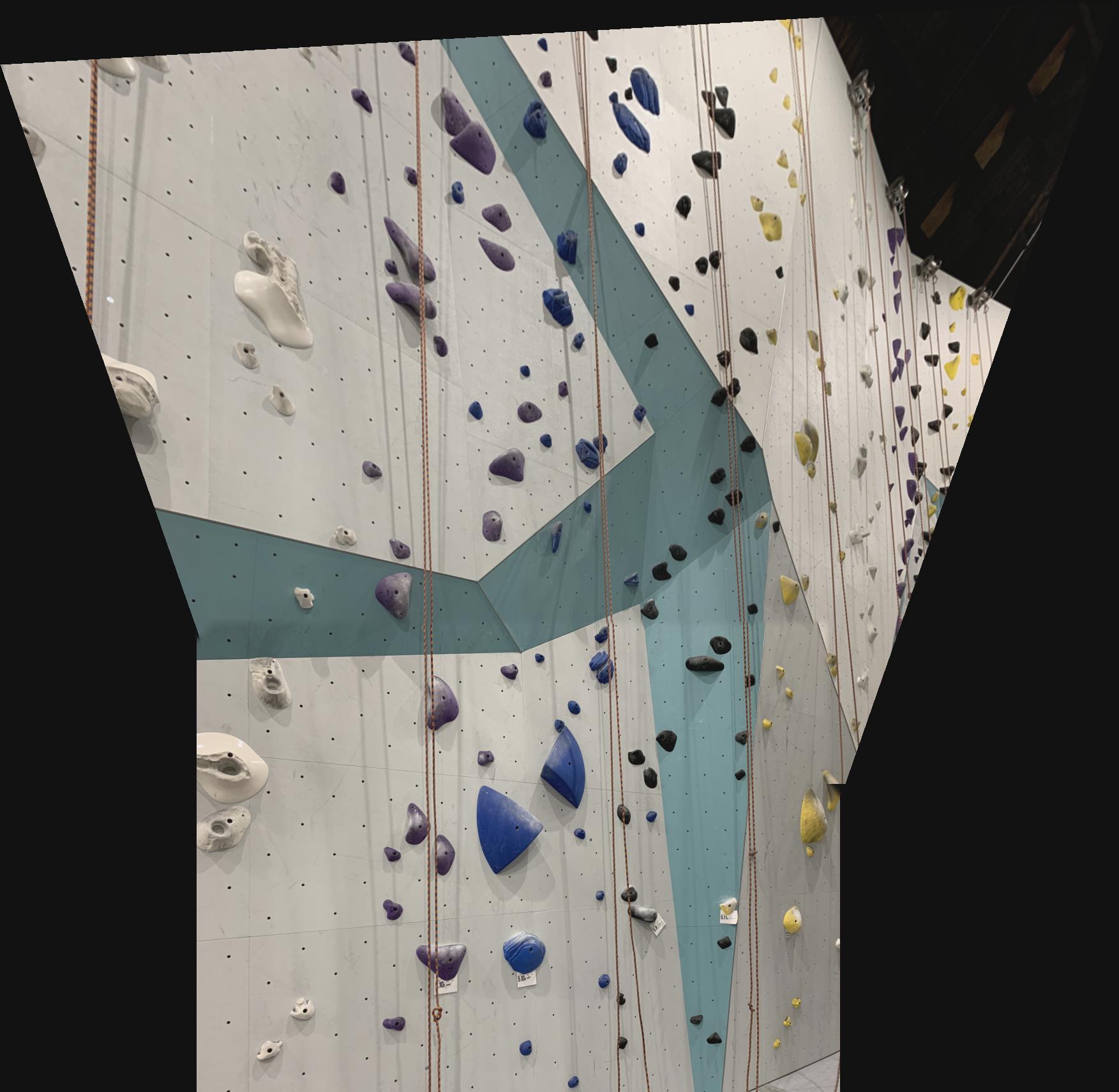
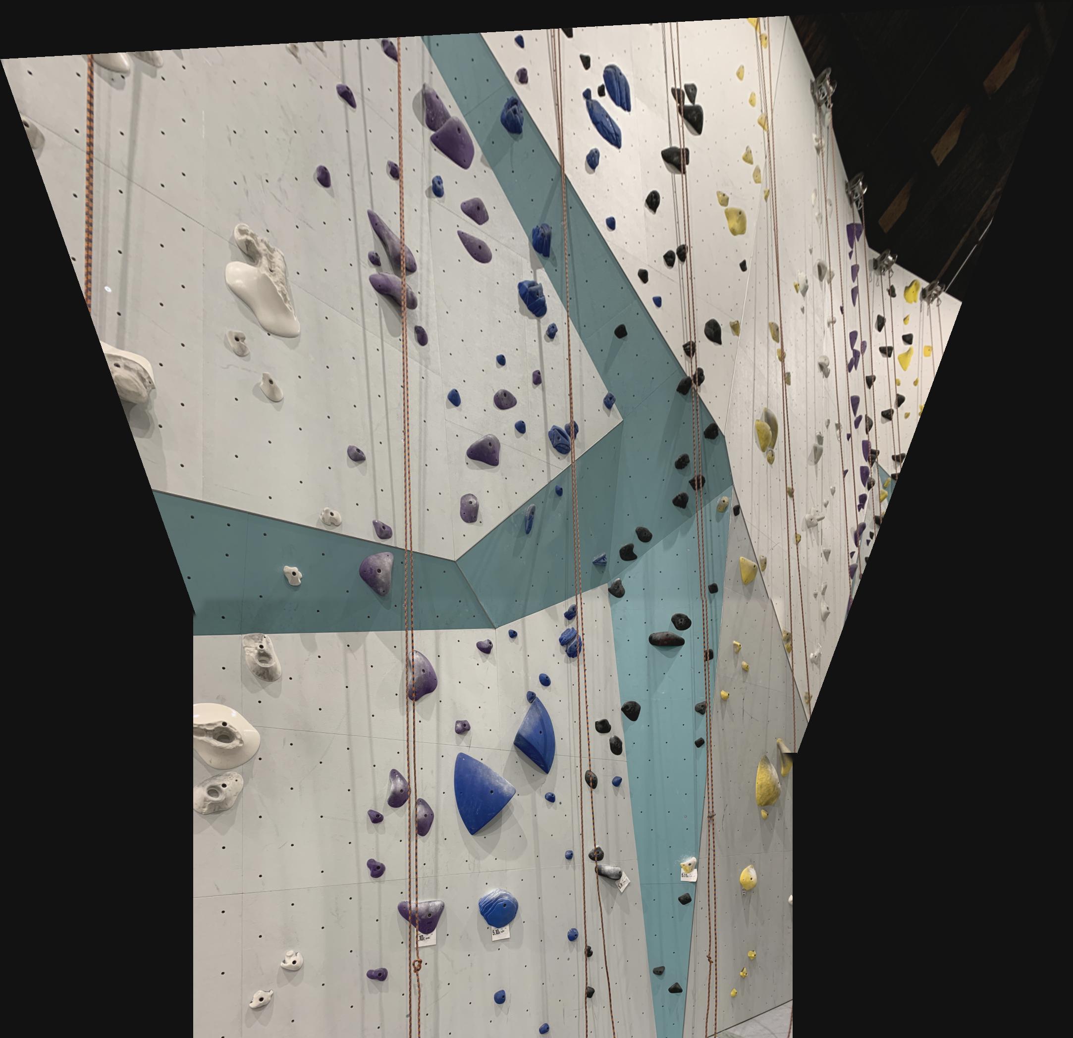
The full toprope wall at Pacific Pipe in a single image:
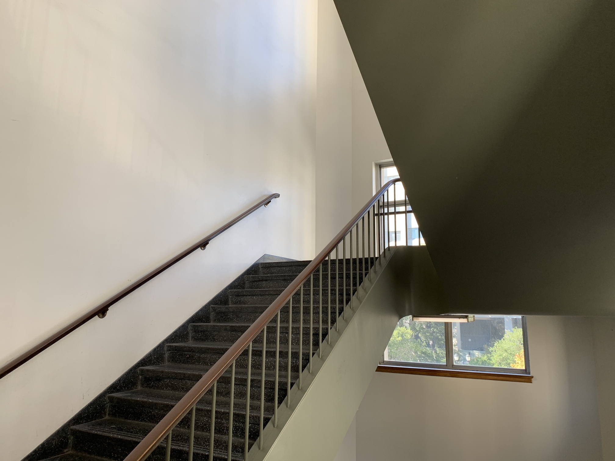
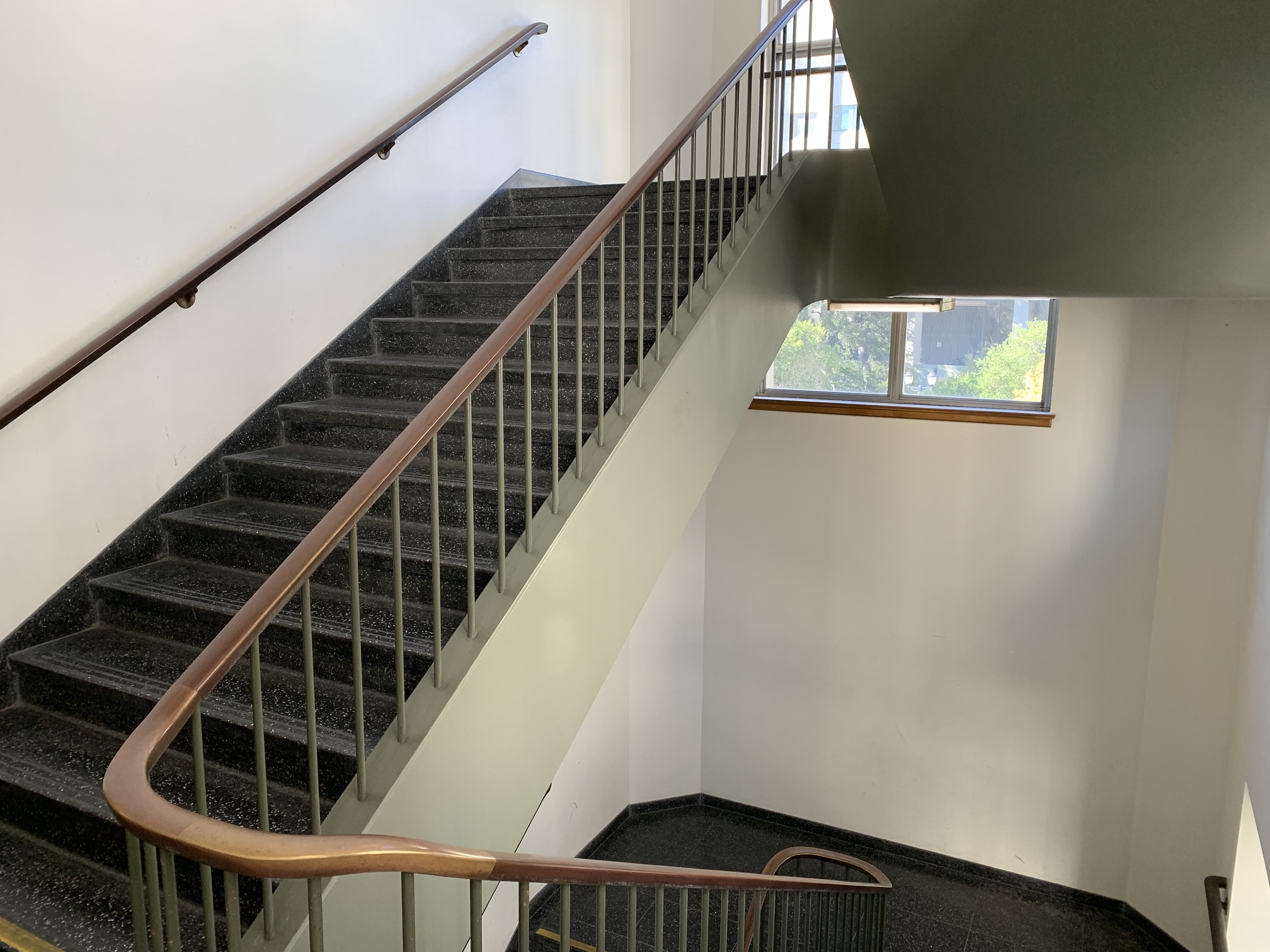
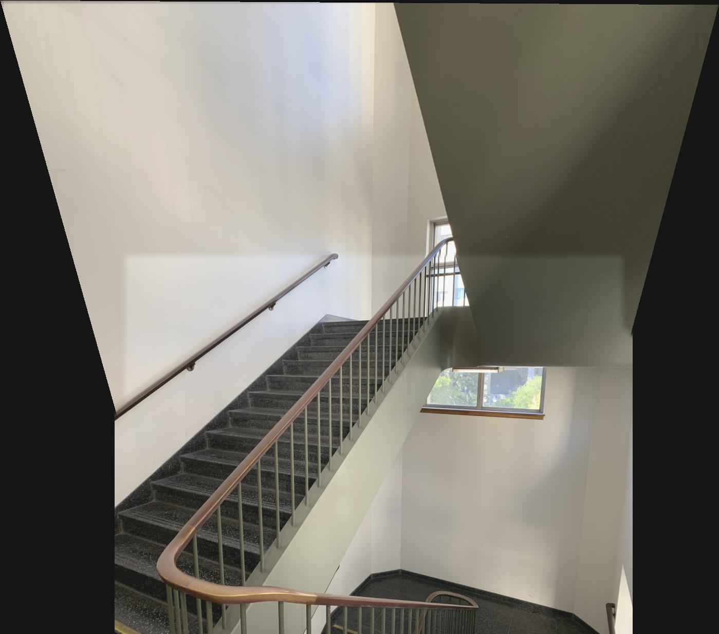
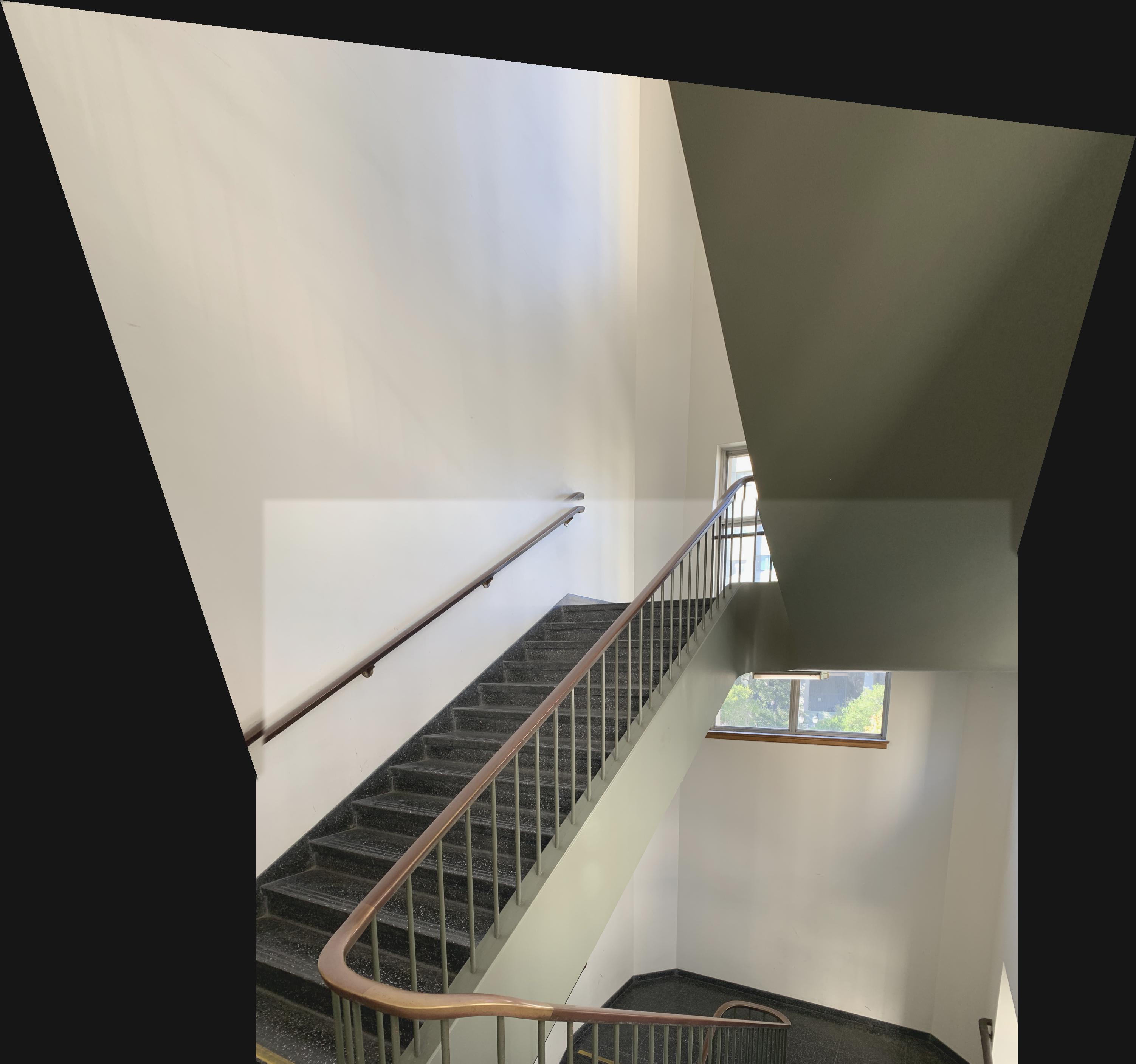
Staircase in Physics building. Here, my phone camera changed settings between the two images, causing drastic lighting differences between the two. However otherwise the image came out well.
What I learned
From this part, I learned that images need to be very well aligned in order to find homographies appropriately. I originally spent a very long time trying to generate a mosaic using another pair of images, but I was unable to do so (or figure out why it didn't work). It must've been because the images weren't taken from the same point, since when I simply took a new image it worked instantly. The lesson is to always try on various data points before drawing any conclusions.
Harris Interest Point Detection
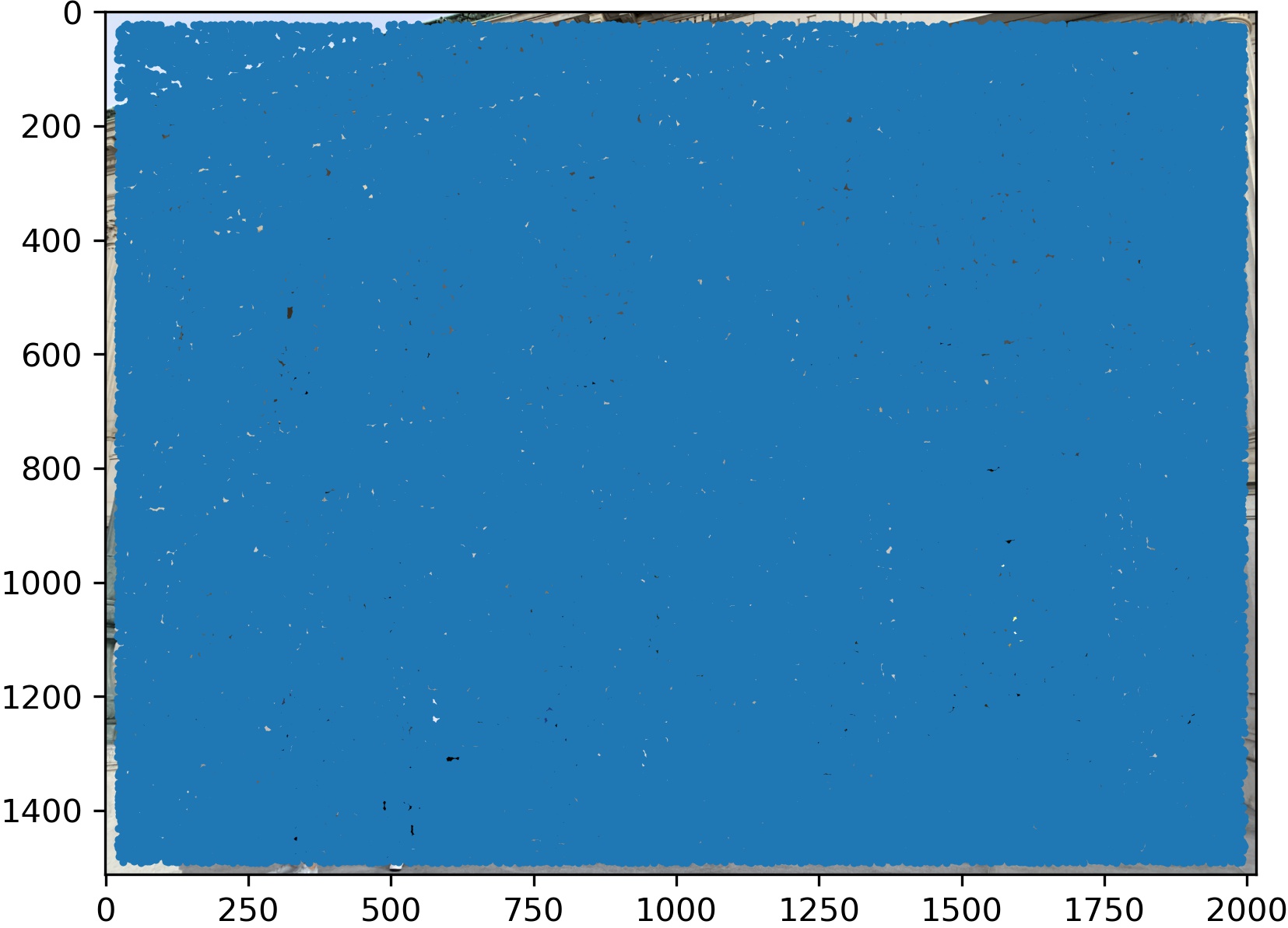
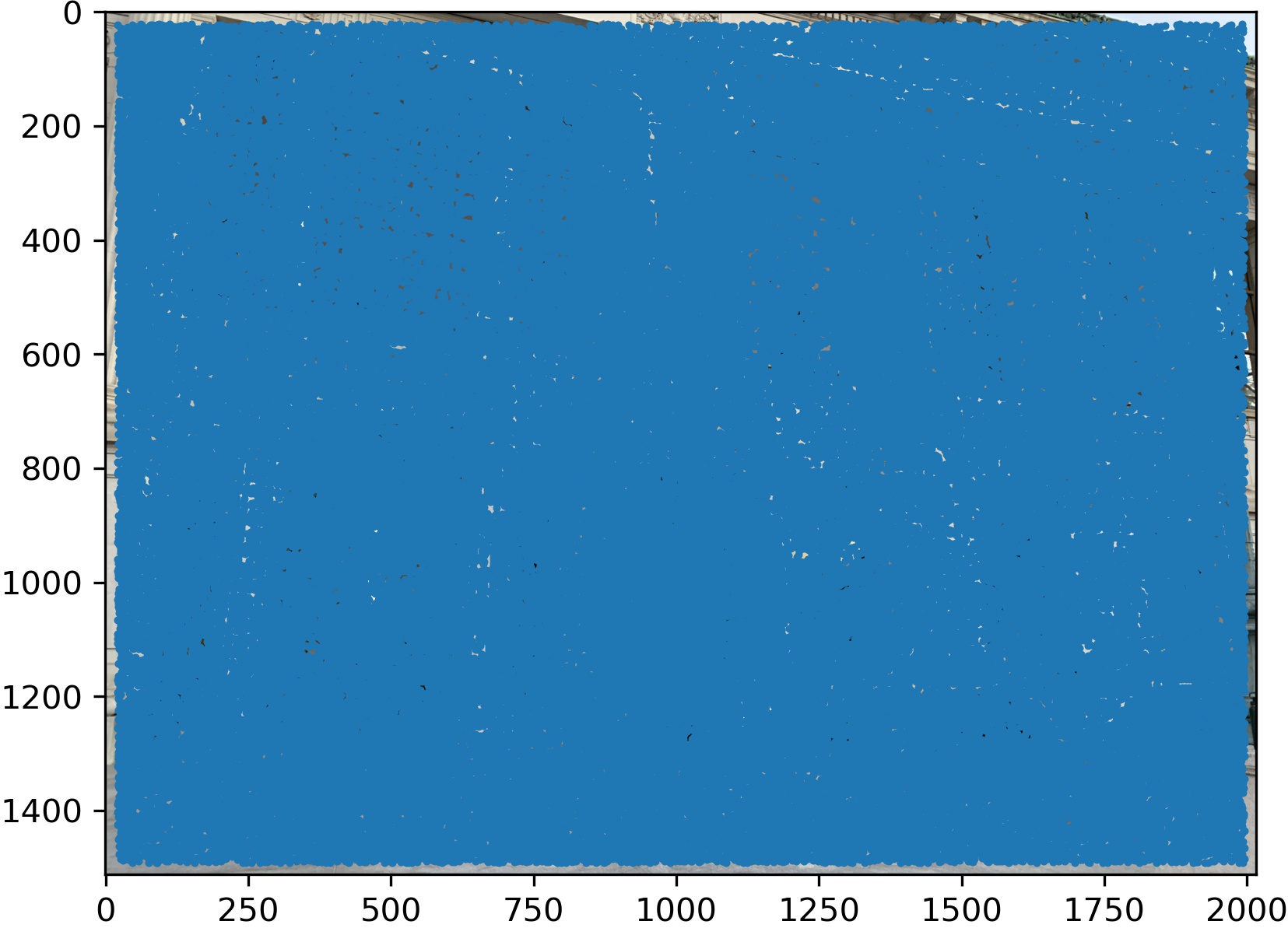
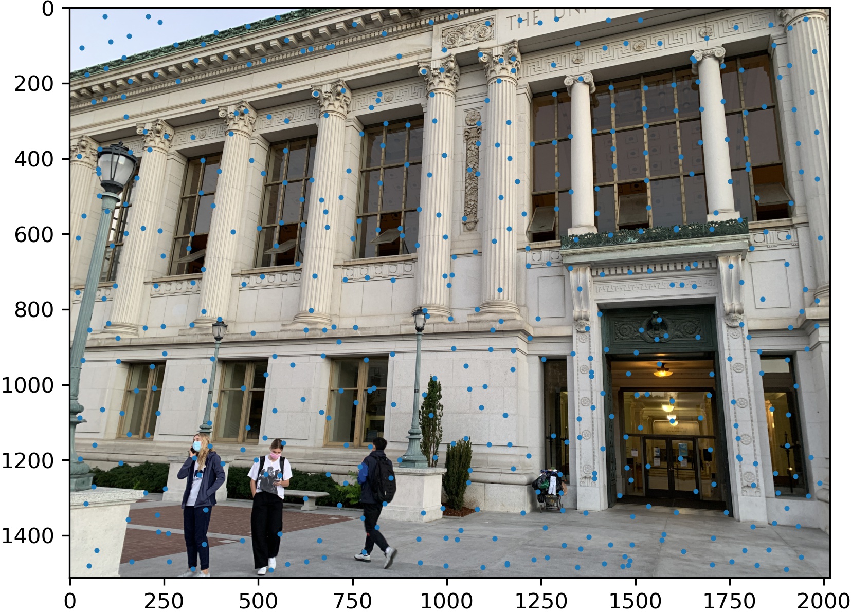
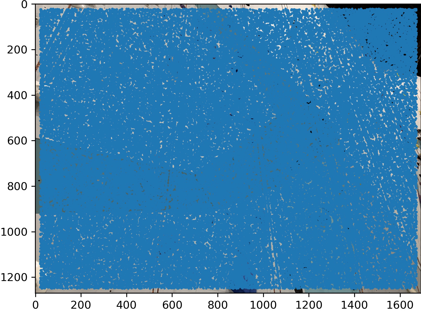
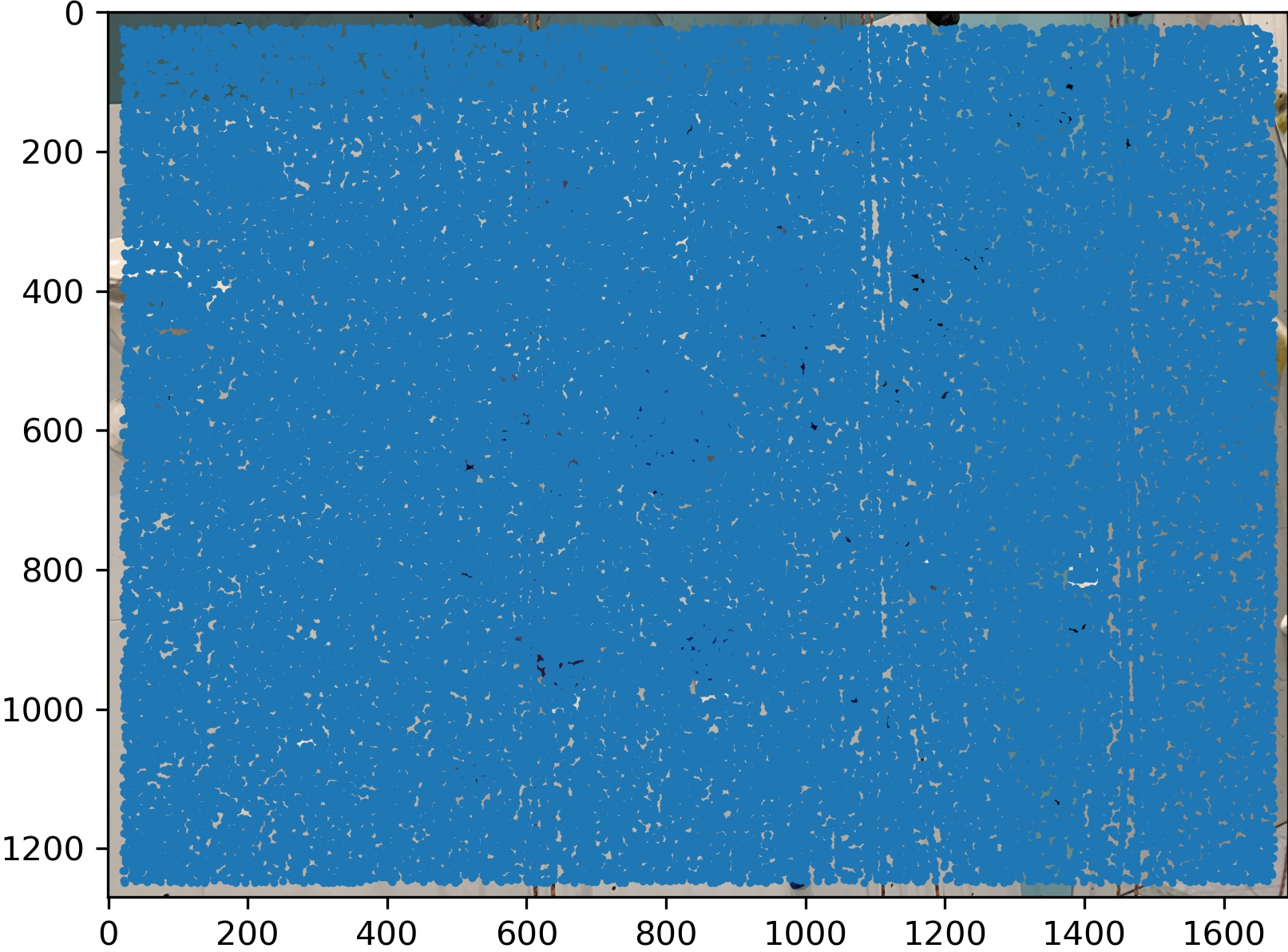
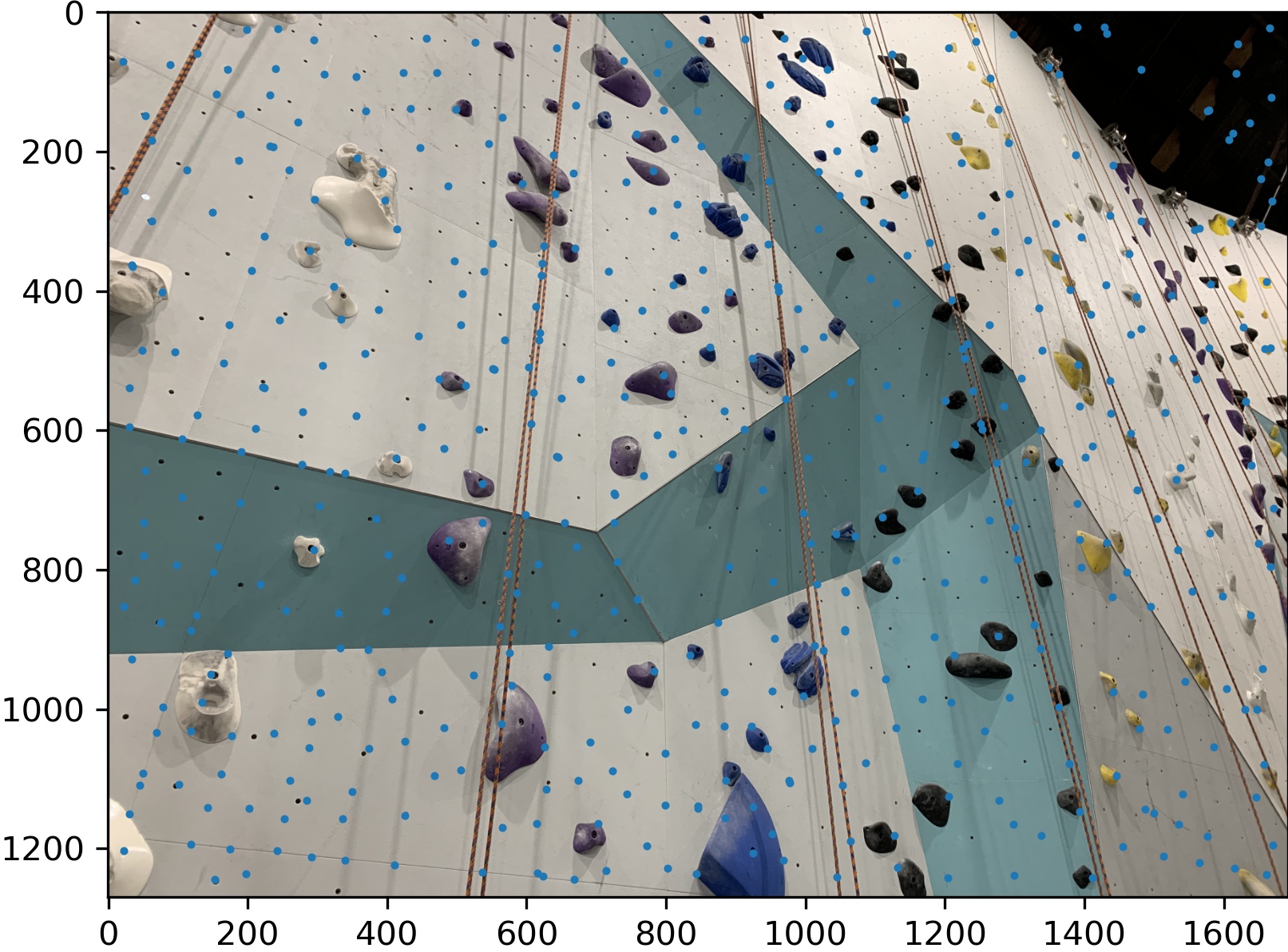
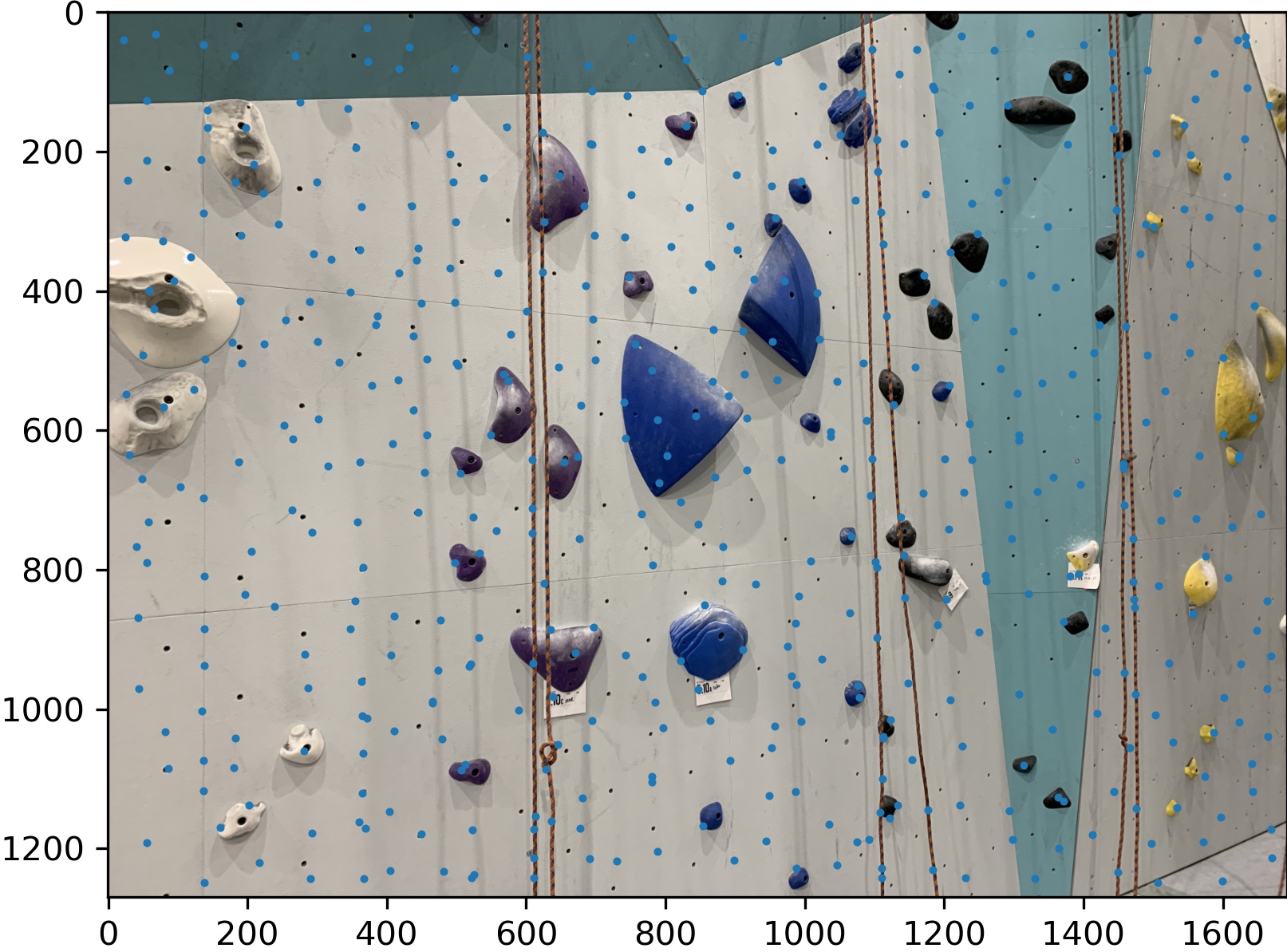
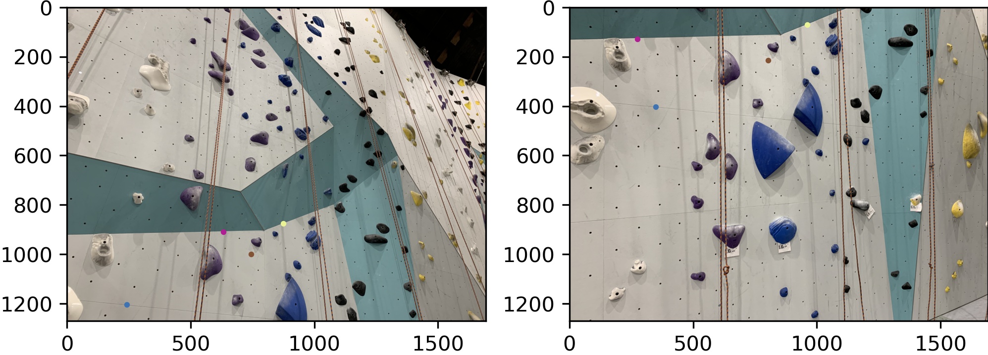
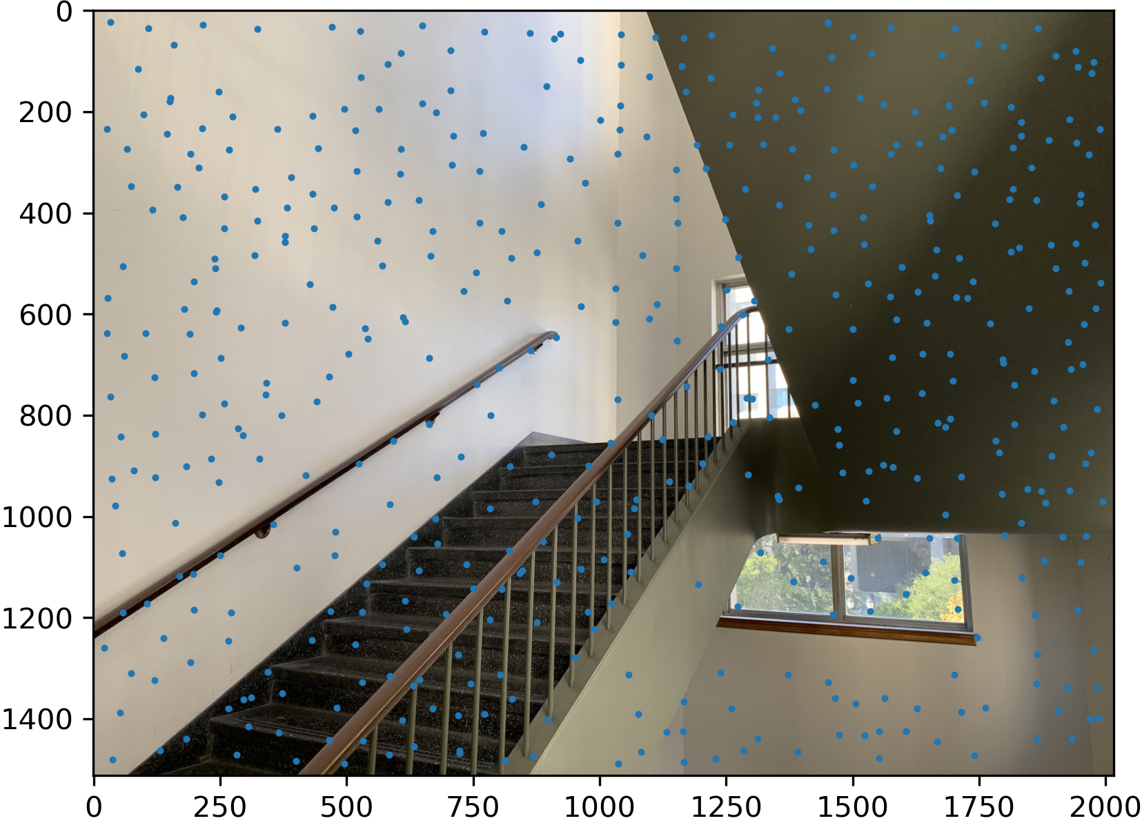
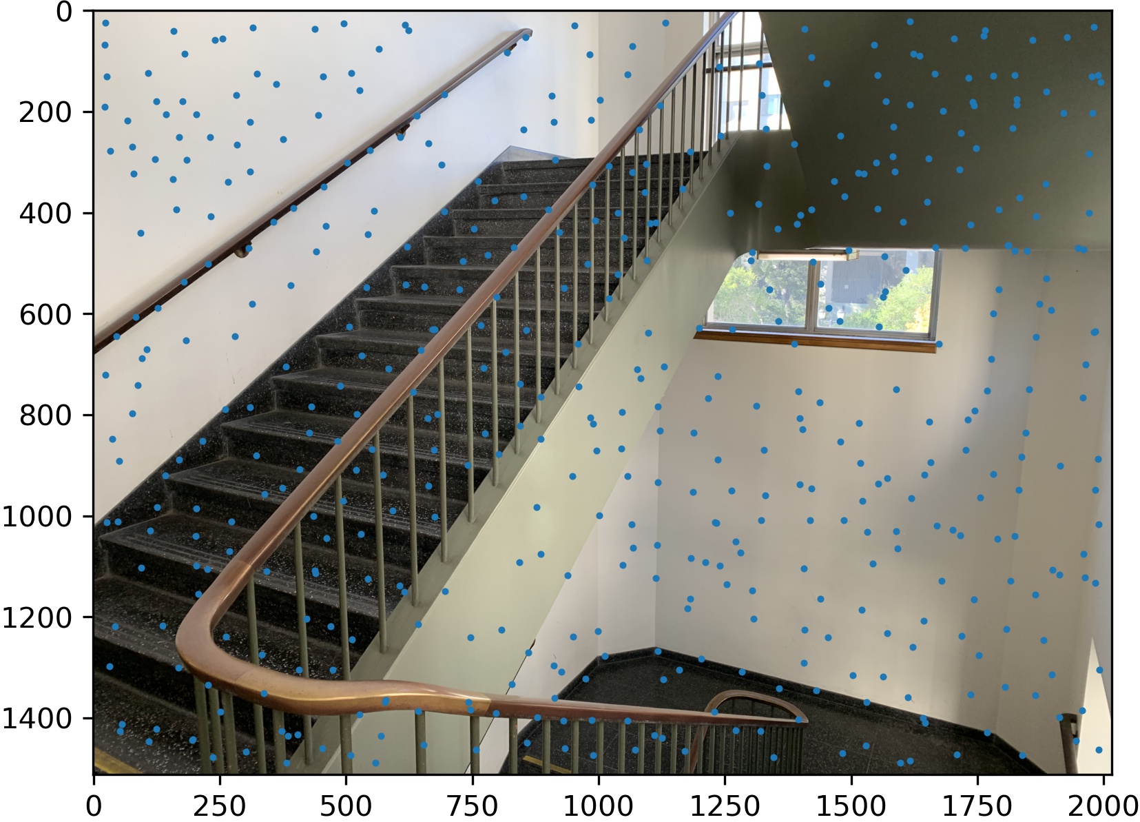
First, we use the provided implementation of Harris point detection to get points of interest on both images. There are an overwhelming number of points though: here's a side by side.
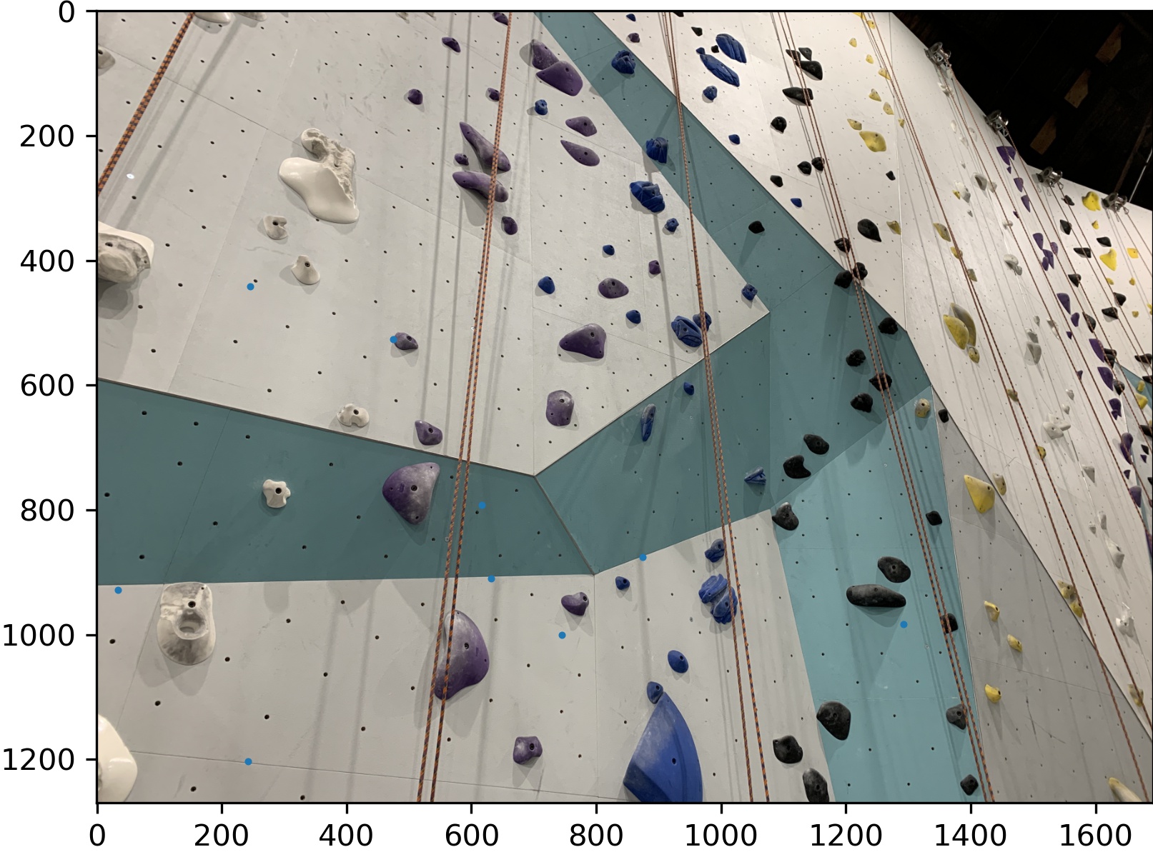
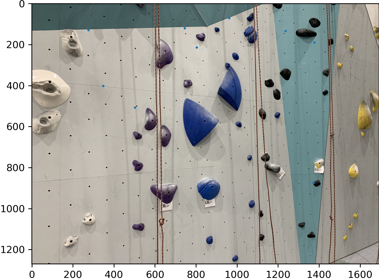
Adaptive Non-maximal Suppression
We need to reduce the number of points by using adaptive non-maximal suppression. We want a more sparsely populated set of points which hold all the most "interesting" corners. We do this separately for each image.
The suppression radius is the minimum radius such that no stronger points (by some robustness factor) are located within that radius.
First, we sort the points by their strength in descending order. We set the suppression radius of the strongest point to be infinity by definition. Then, for each point, we check stronger points than it and update the suppression radius accordingly.
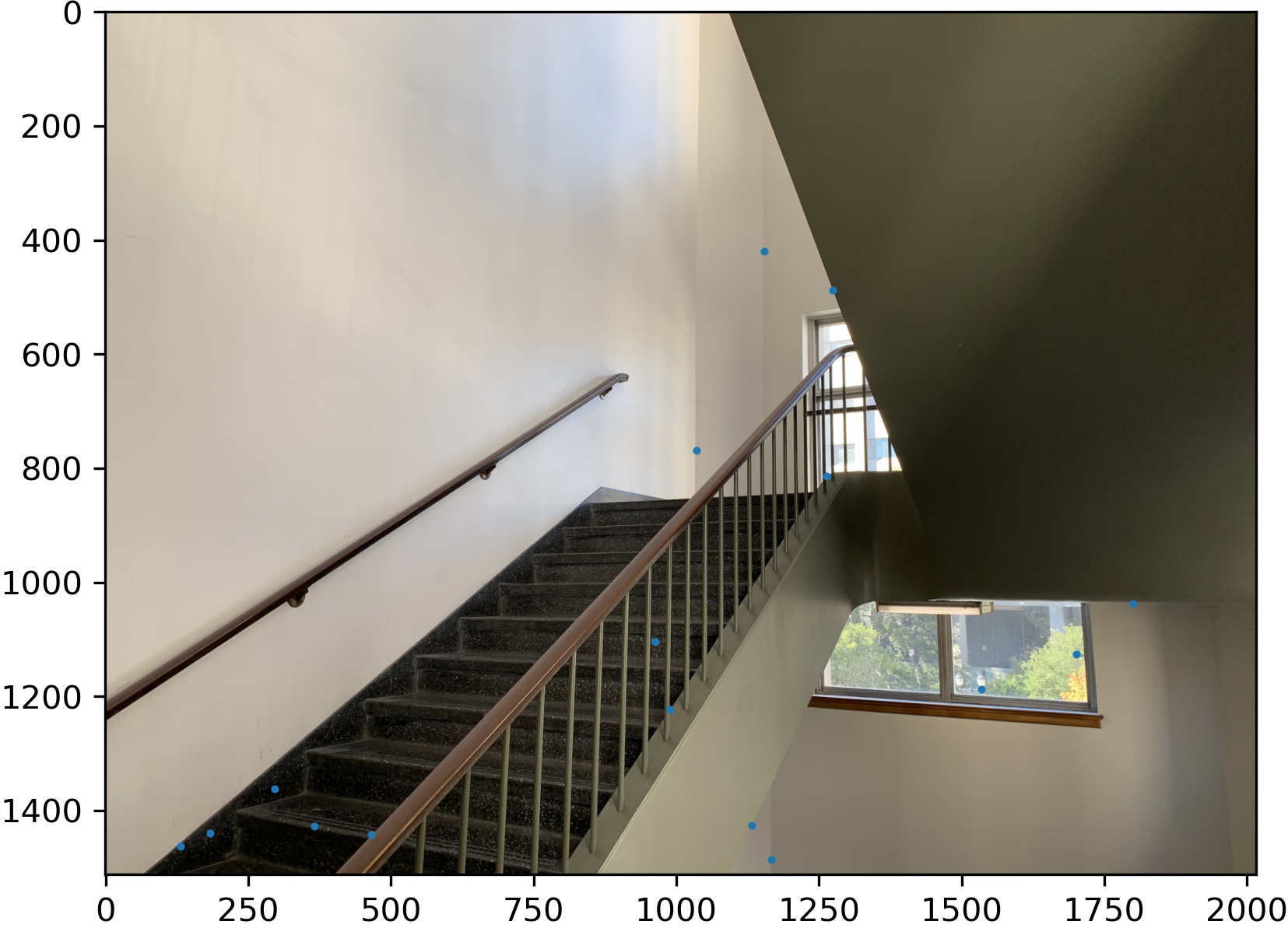
Once we've done this for all points, we simply return the first 500 points with the largest radii.
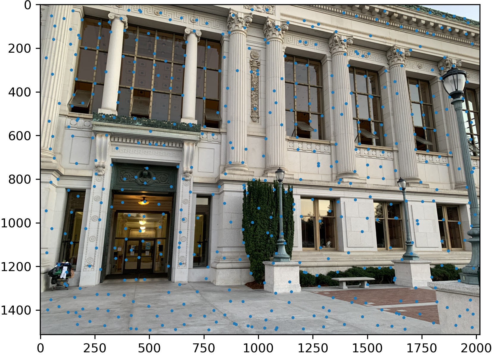
Looks good!
Sampling Point Descriptors
We have to get a feature descriptor for each point. To do this, we simply downsample a 40x40 patch around the point to an 8x8 patch. Here is one such patch:
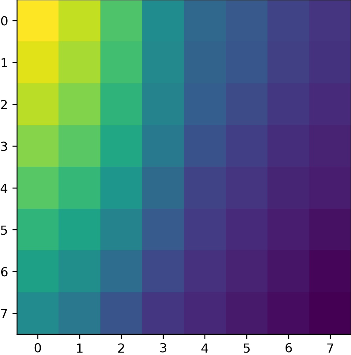
We also normalize each patch to be mean 0 and standard deviation 1.
Feature Matching
Lowe Thresholding
First, we use Lowe thresholding to help remove outlier correspondences. We make use of the fact that a good match has a much better best match than the second best match for a given point.
Using a KNN algorithm, we find the first and second best matches for every point. Then, we threshold based on the ratio (1-NN loss / 2-NN loss) which should be less than 0.5.
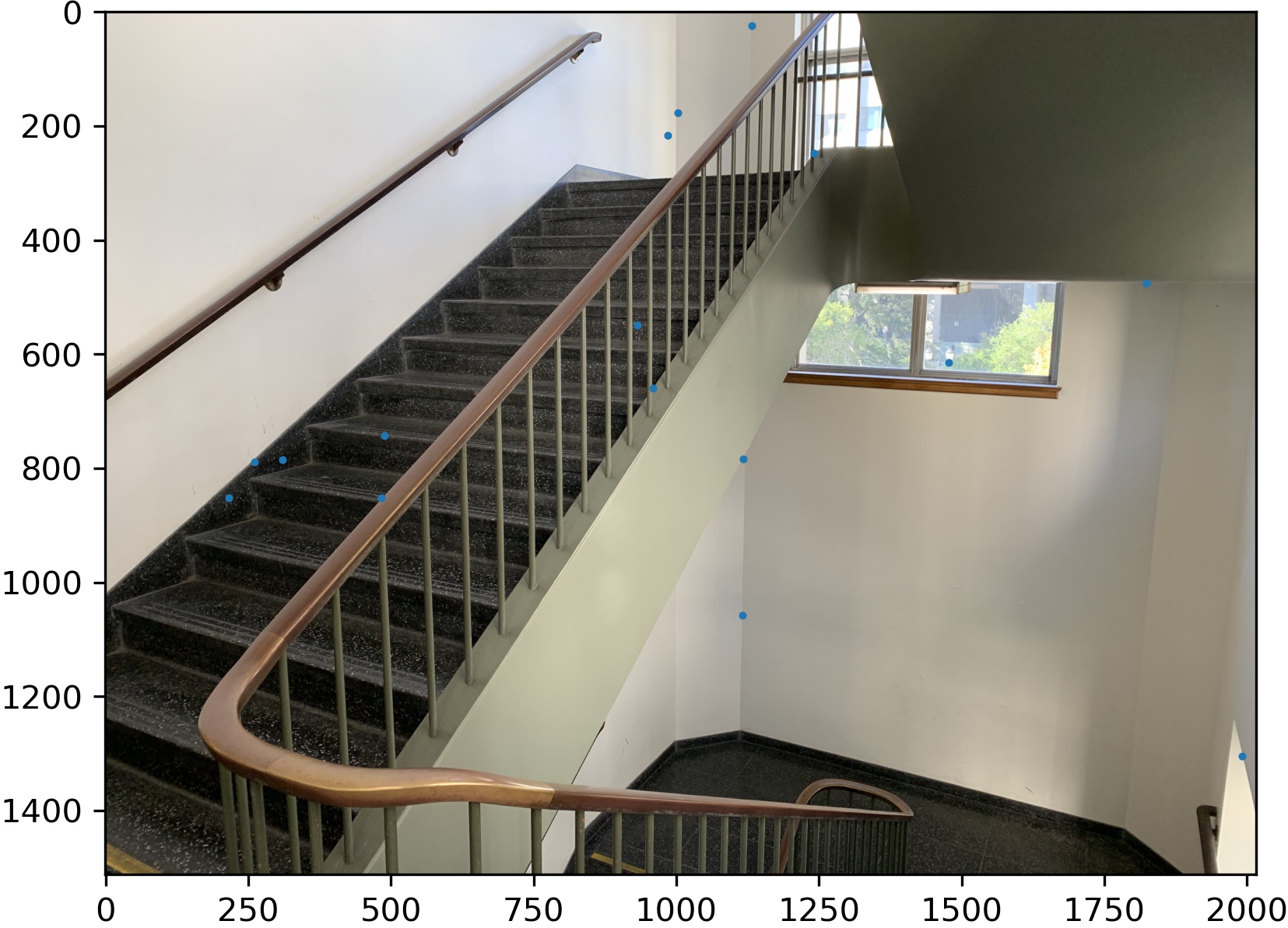
This leaves us the following points:
RANSAC
This still isn't perfect, so we need to run RANSAC in order to get the optimal homography. We randomly sample 4 points, then transform all the points based on those 4. If this is the best homography so far (the most correspondences match) then we use these matching correspondences and calculate another homography. We repeat this process for 1000 iterations.
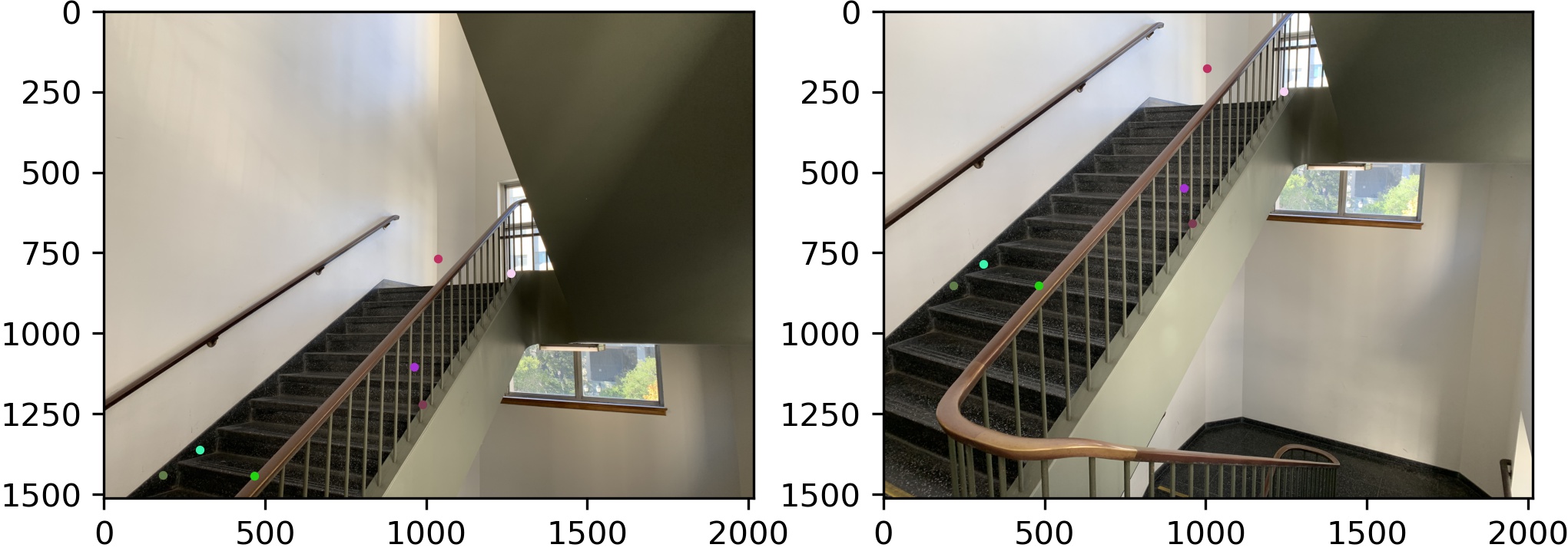
This leaves us with the following corresponding points:
Combining the Images
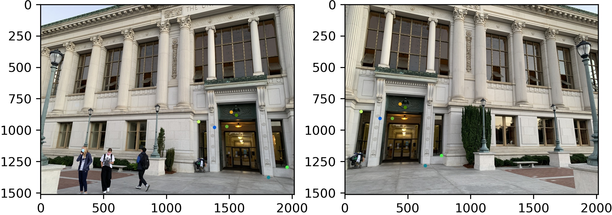
Finally, we follow the steps described earlier to combine the images using this new homography. Let's compare some of the manually aligned and automatically aligned images.
The left image is manually aligned, while the right image is automatically aligned.
Intermediate Results for Climbing Wall and Stairwell
Climbing Wall:
Stairwell:
What I Learned, Part 2
I found the automatic feature matching very interesting. Implementing both Lowe's method and the adaptive non-maximal suppression were both novel ideas to me. I liked how we could use Harris corners to get points which were more easy to obtain and more abundant than when manually picking points.