|
|
|
|
|
|
|
|
||

|
|
|
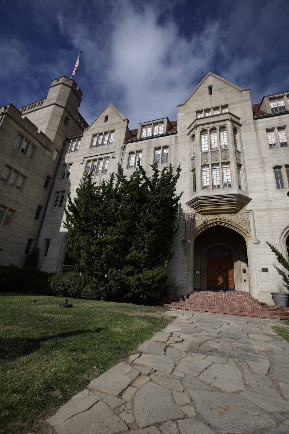
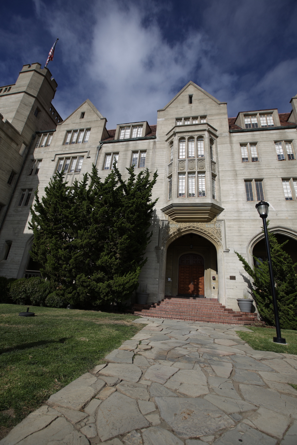
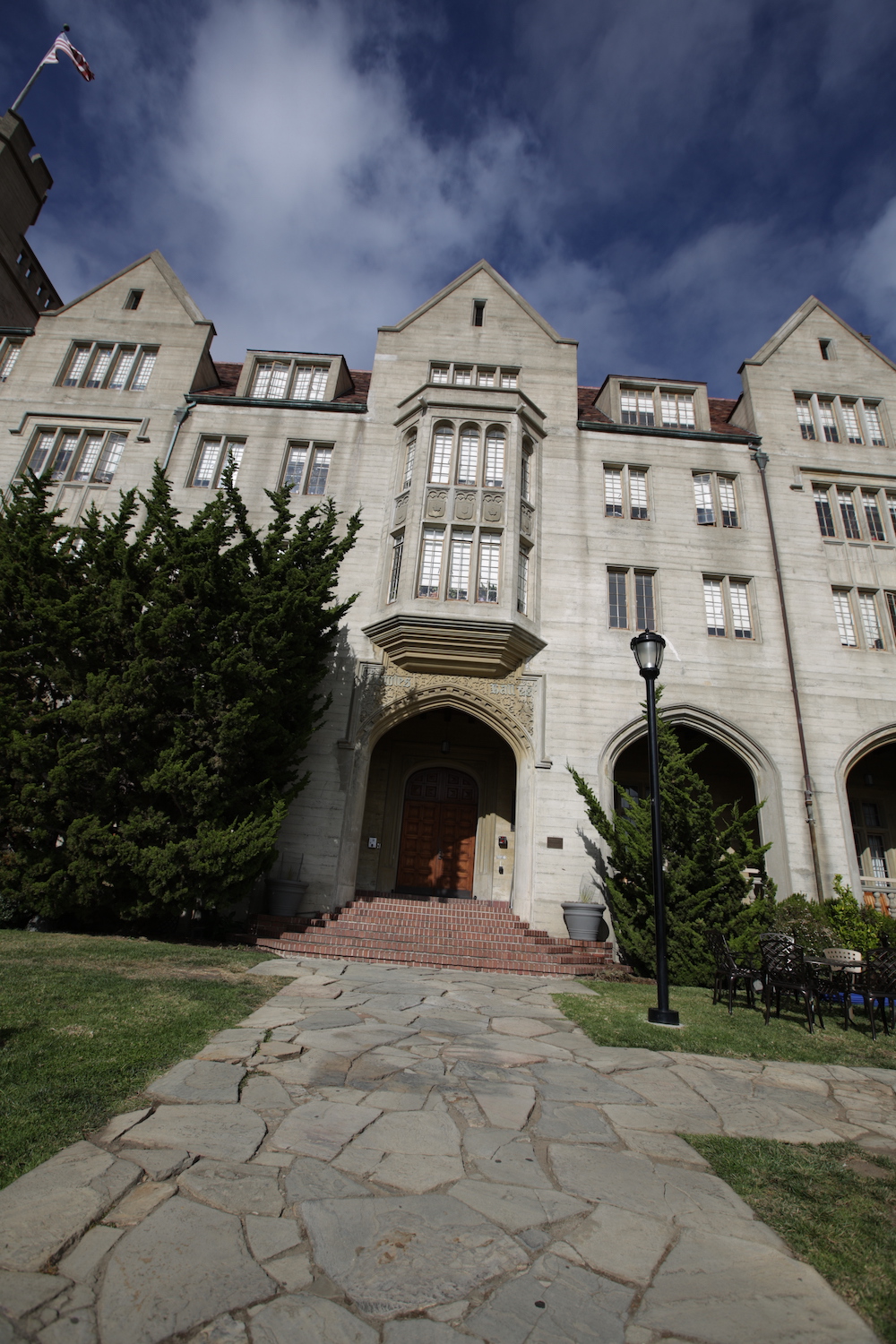
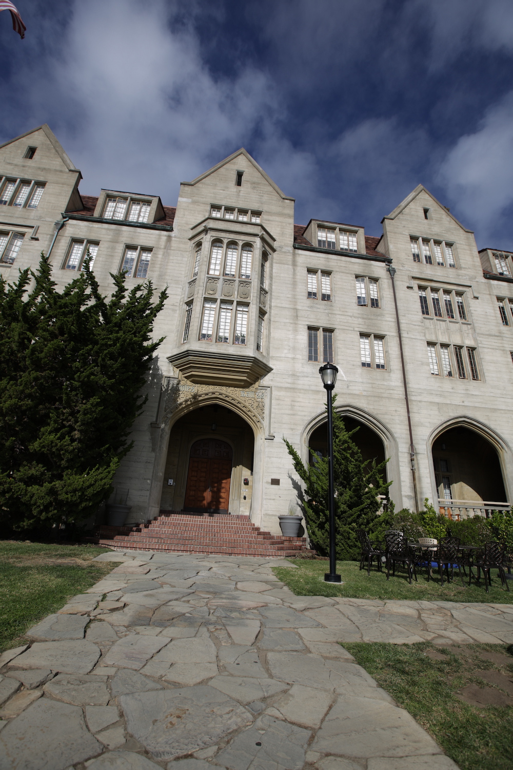
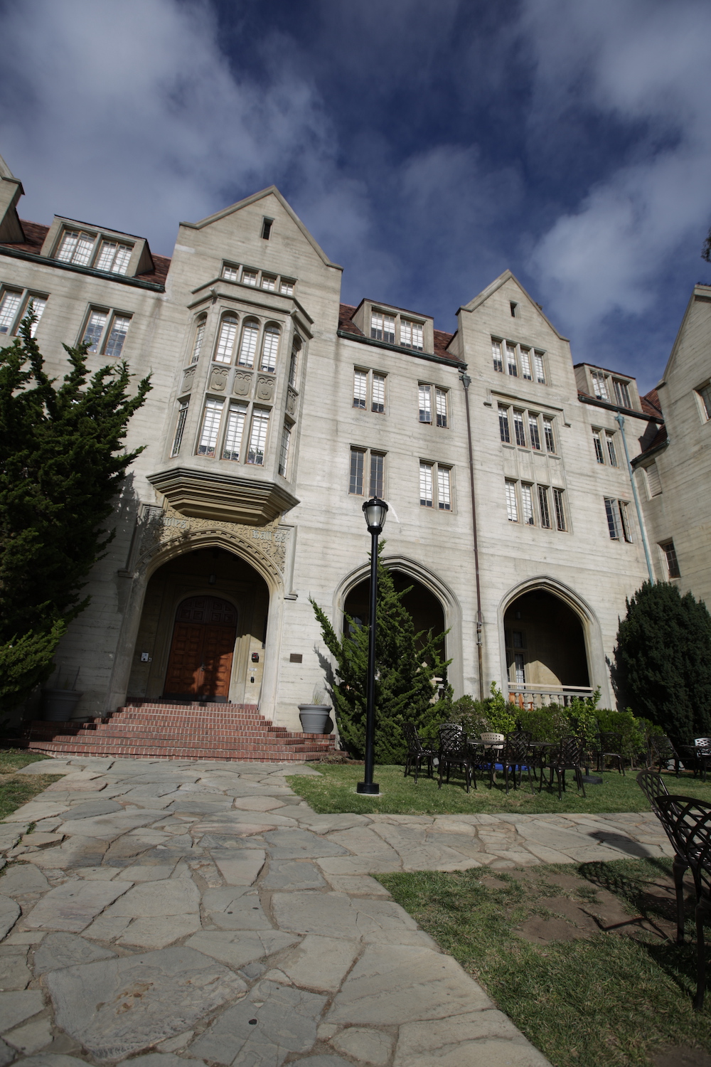
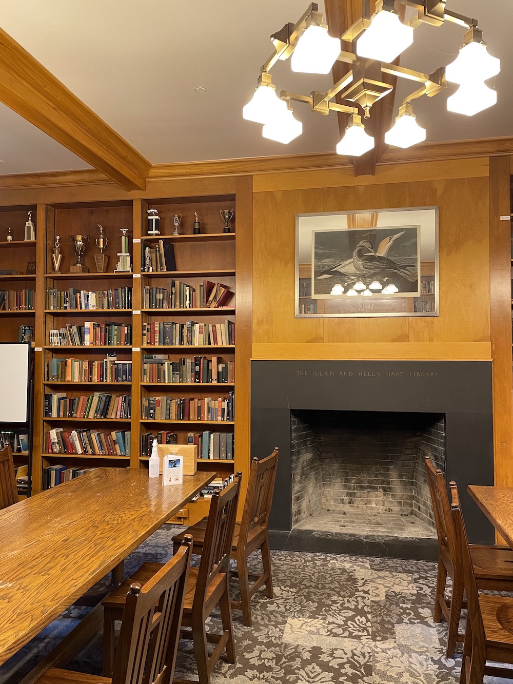
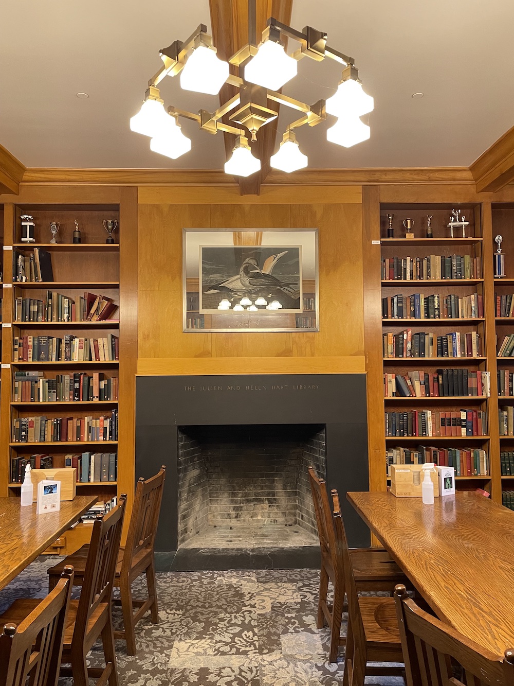
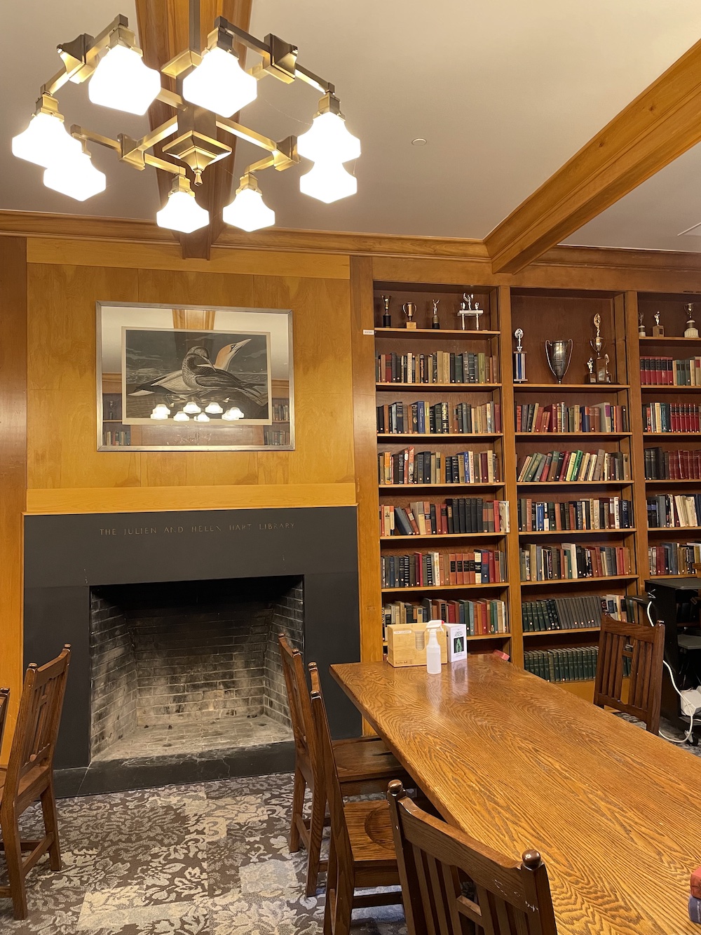
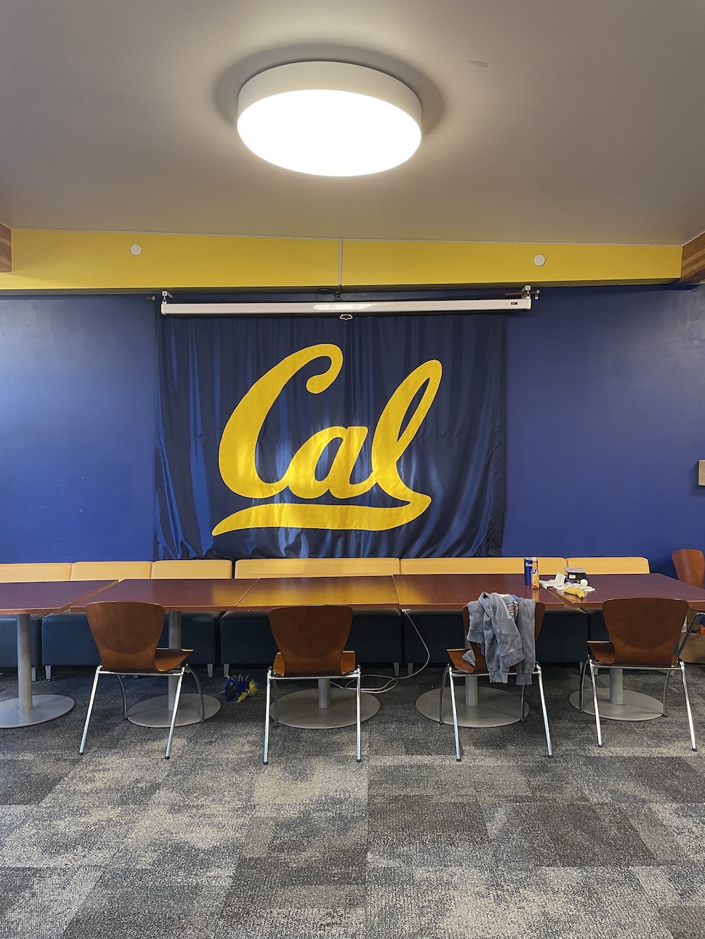
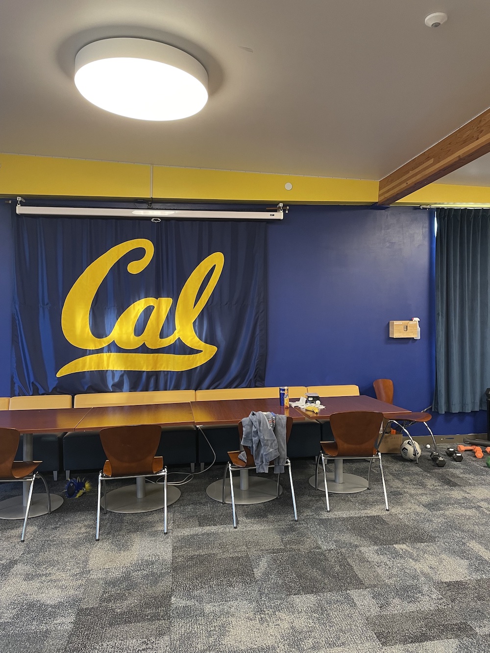
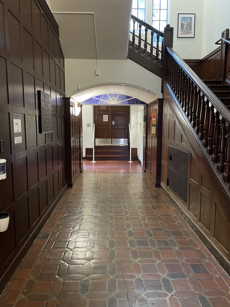
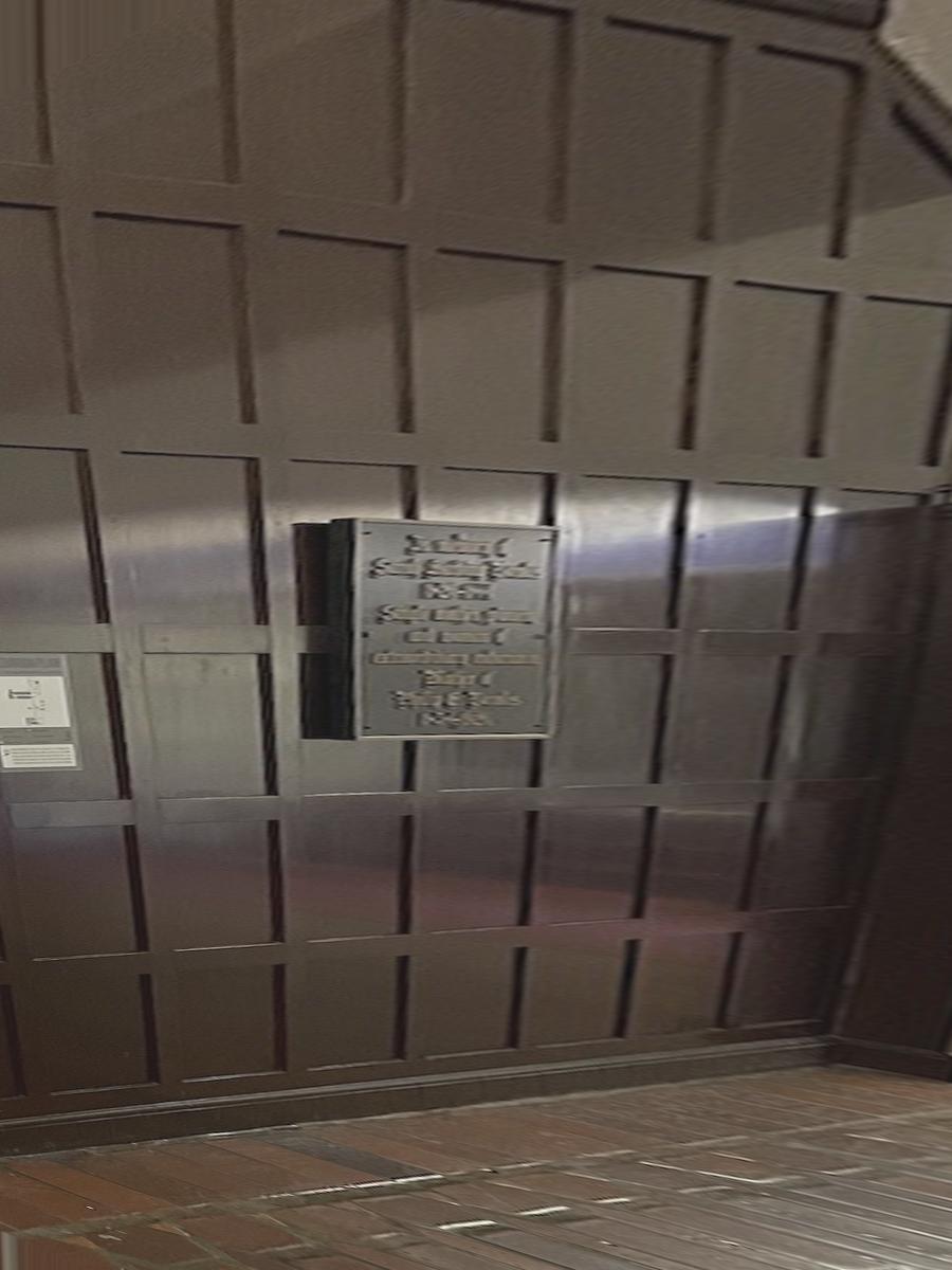
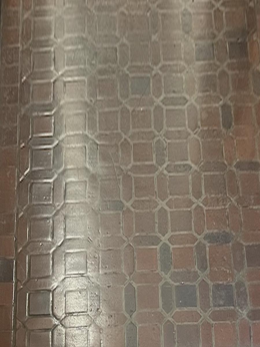
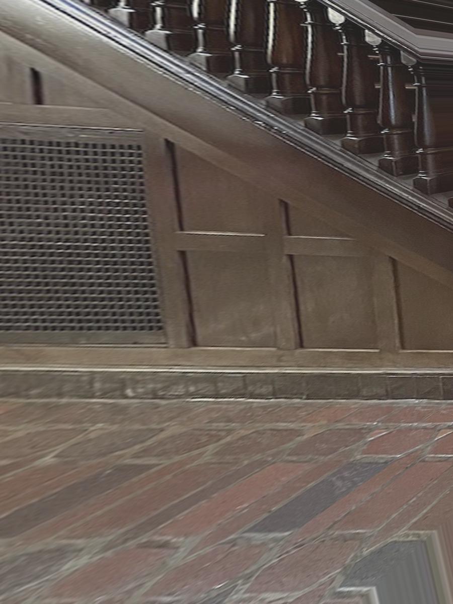
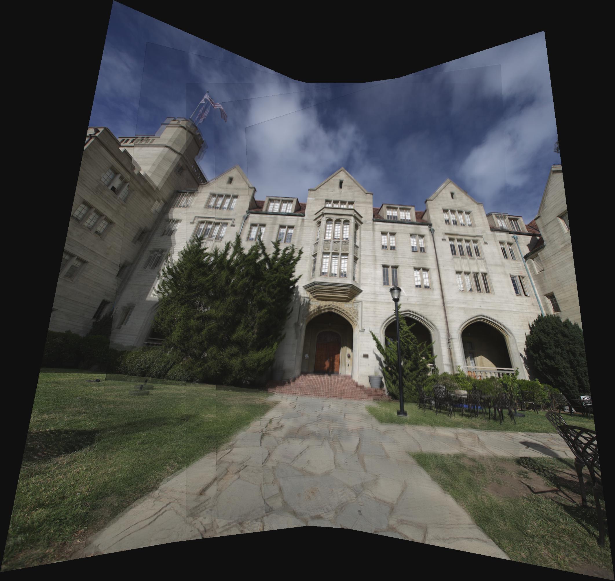
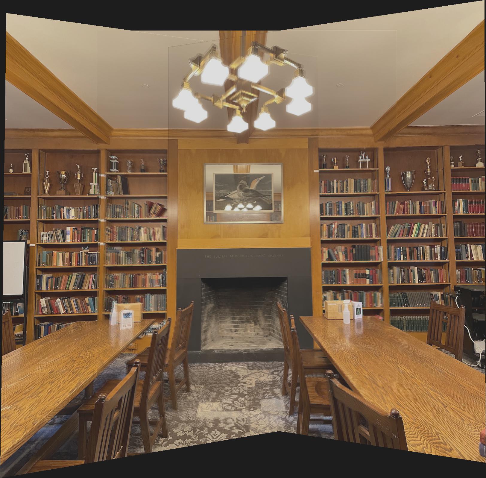
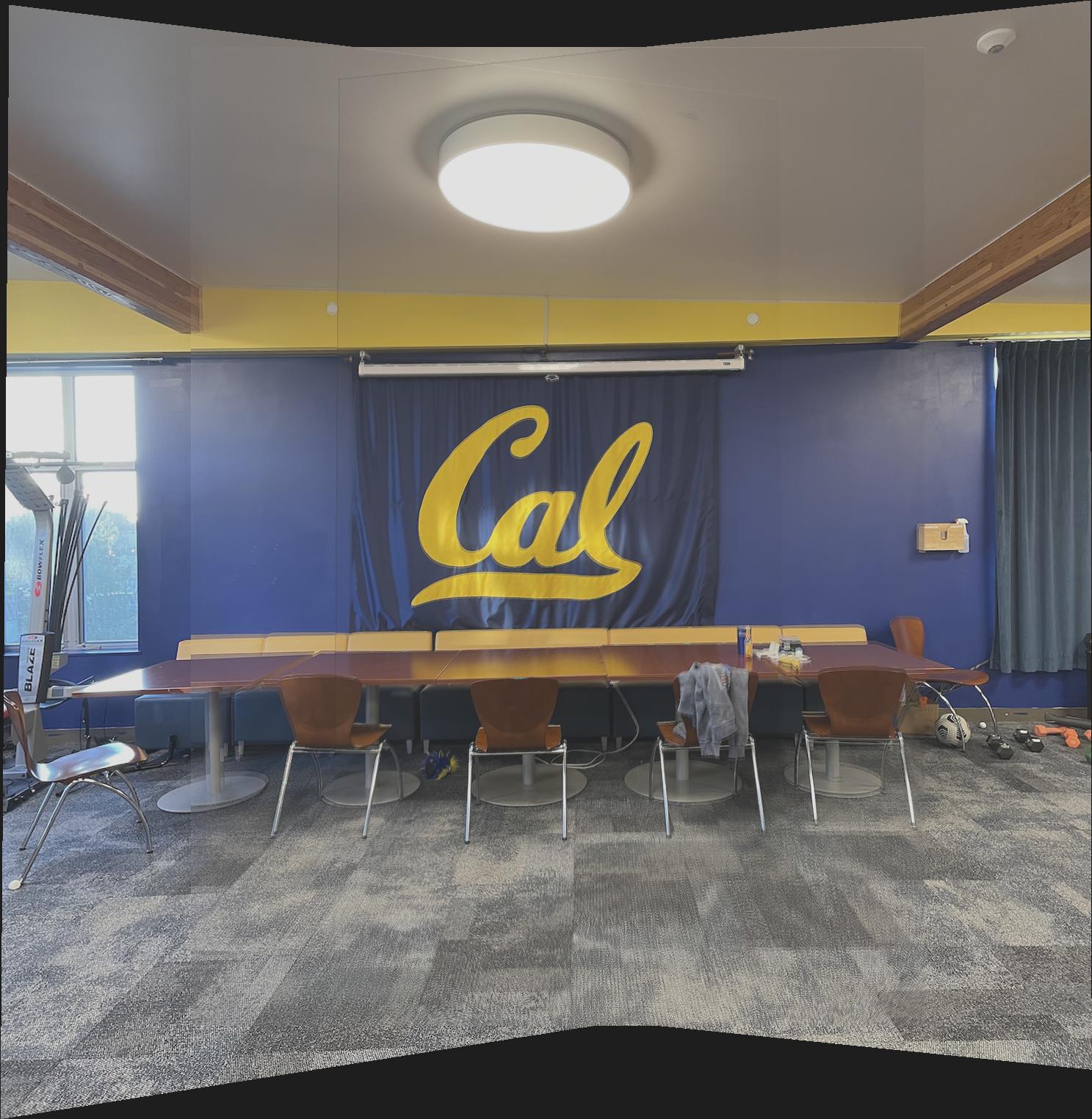
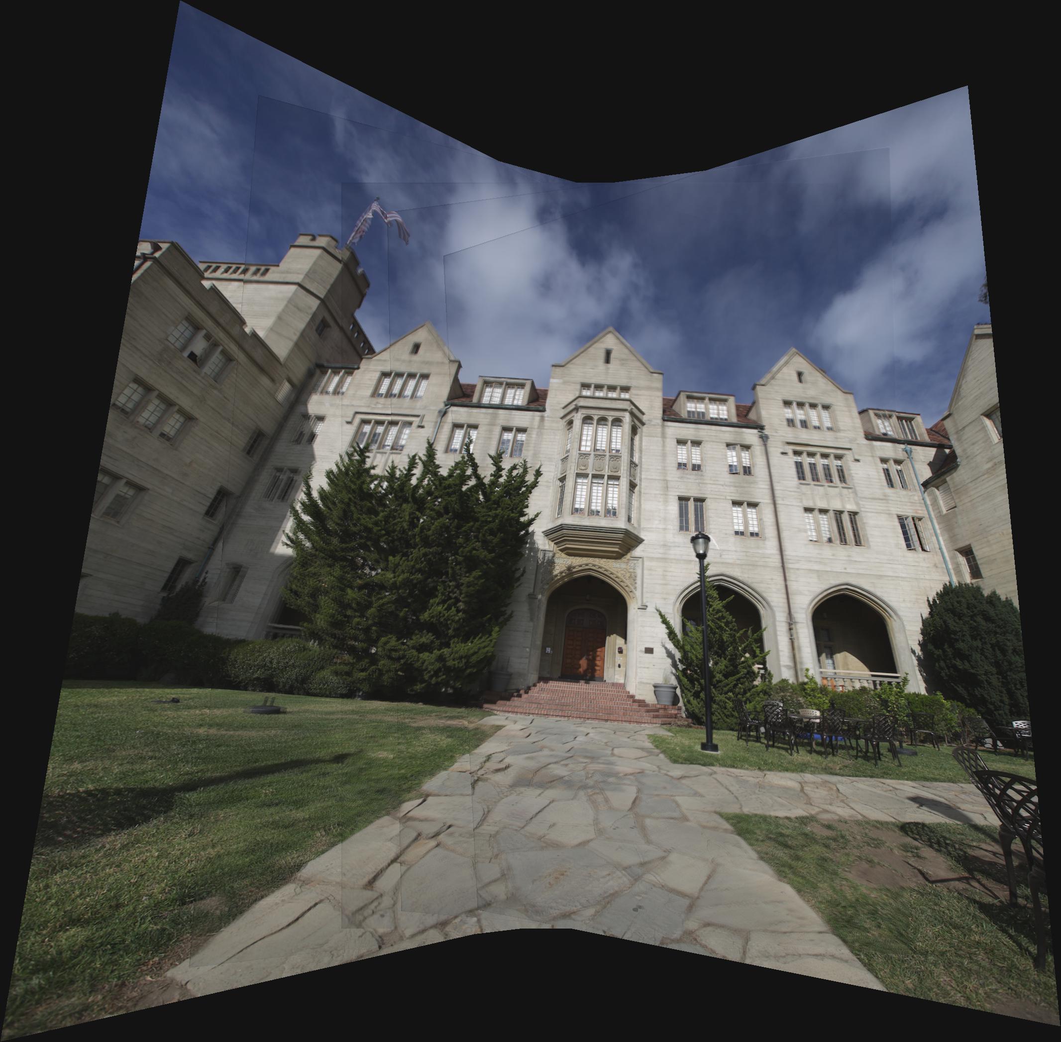
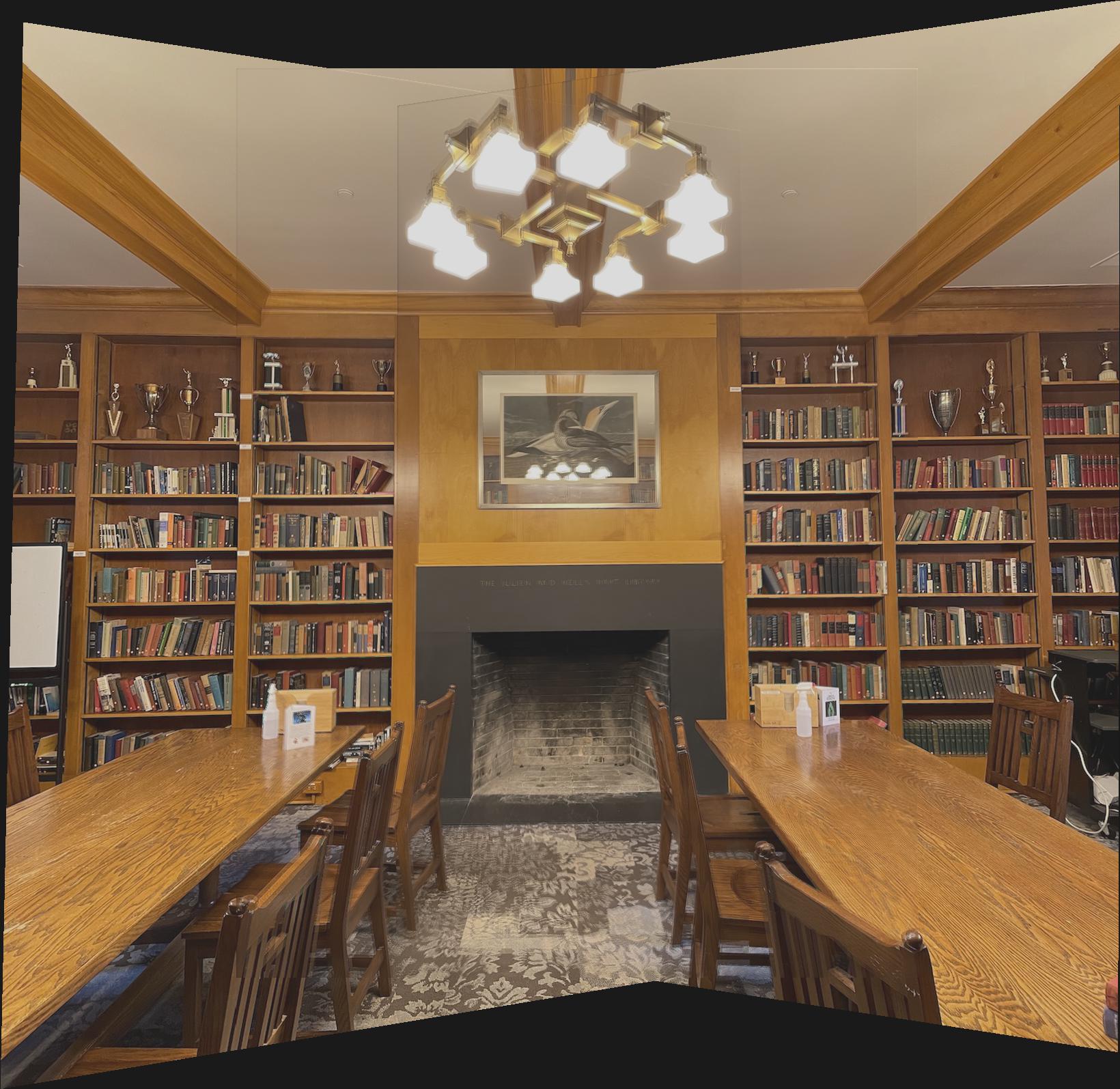
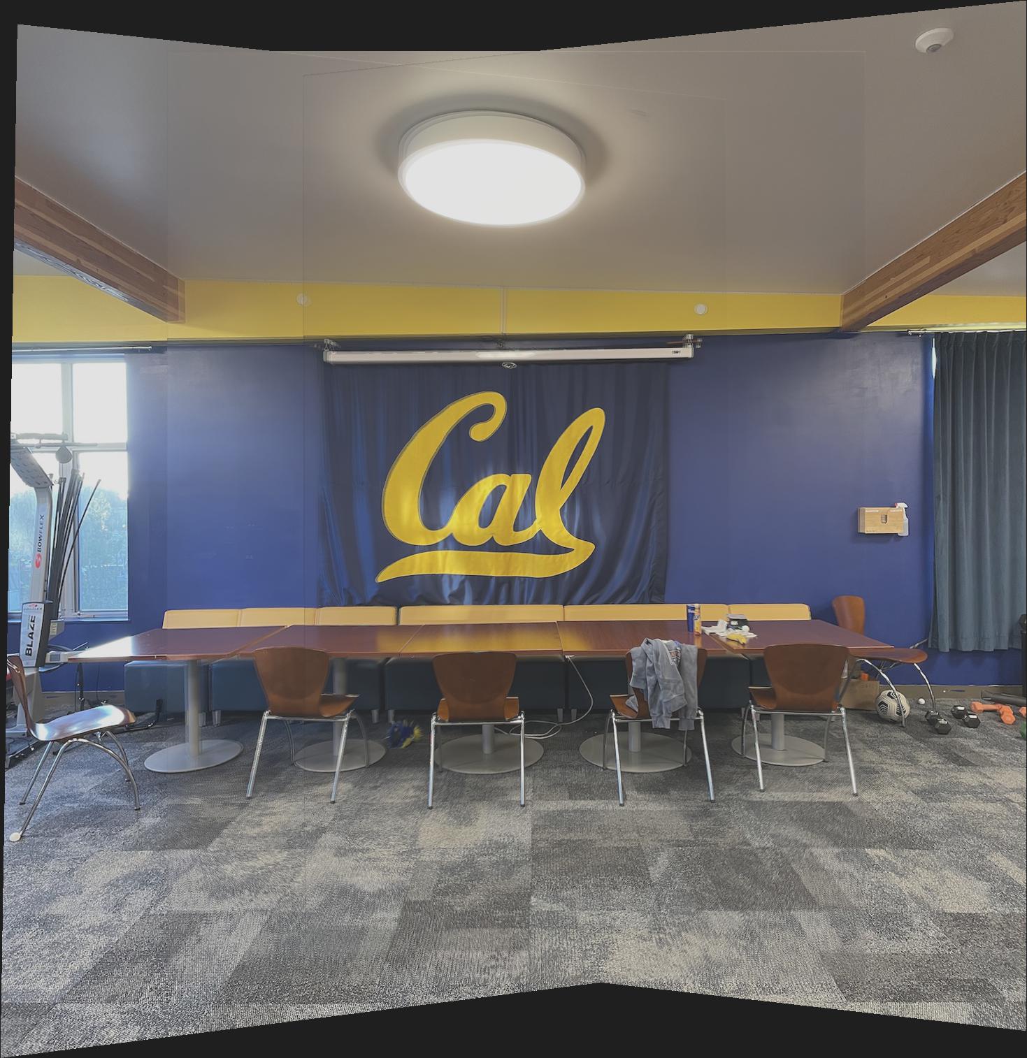
The three scenes that I shot to make a mosaic out of are Bowles Hall (note the flying flag, this will make the mosaic in that region worse than if the photos were taken on a non windy day), and two other rooms inside the hall. The photos of each set were taken so that a large part of them overlapped and correspondences could be defined between the images.
|
|
|
|
|
|
|
|
|
|
||
|
|
|
|
We seek to solve for the projective transformation matrix H in
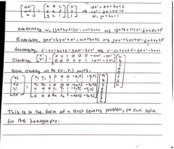
All of the images are warped as defined by the homography that was solved for using least squares in the above equation. Inverse warping is used to fill in color.
In order to warp an image so that a plane in the image is frontal-parallel, I define a correspondence between a square on that plane and a manually defined square in the center of the image.
|
|
|
|
First, all the images in the scene are warped to the middle image by computing the homographies to the middle image, and warping the whole image with appropriate image boundaries computed using the corners. Then, the total image boundaries are computed by the range of where the corners of each image land after warping with the homographies. Each image is placed (from left to right) into the total image by computing the offset between the image and the top left corner, and using a laplacian stack to blend the overlapping regions. From below, can see that the images are very well aligned in the middle region where the correspondences are defined, but degrade slightly as we move away from the center.
|
|
|
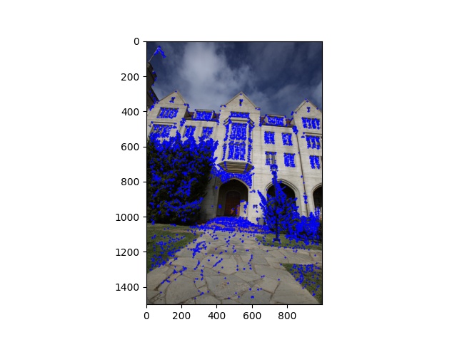
Using the provided algorithm for computing Harris corners, the following result was attained (image of Harris corners overlaid on the image). A threshold value of .1 was chosen as the minimum intensity of the peaks.
|
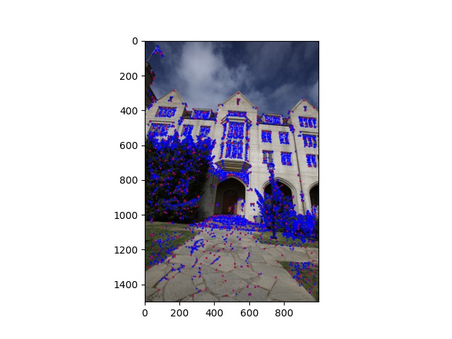
Following the description in the paper, the 500 interest points (in red) with the largest minimum suppression radius are chosen , where minimum suppression radius is defined by

where x_i is a 2D point in the image and I is the set of all interest points. c_robust is set to 0.9 as in the paper.
|
At each interest point, an 8x8 patch is sampled from a 40x40 patch centered at the interest point. The patch is then normalized to have mean 0 and standard deviation 1.
The one and two nearest neighbors of every interest point feature in the first image to every interest point feature in the second image is computed (nearest neighbor based on SSD error). The pair of the first image interest point feature and its nearest neighbor in the second image is considered a match if the ratio of the first and second nearest neighbor errors is less than 0.5.
The RANSAC algorithm was implemented as follows:
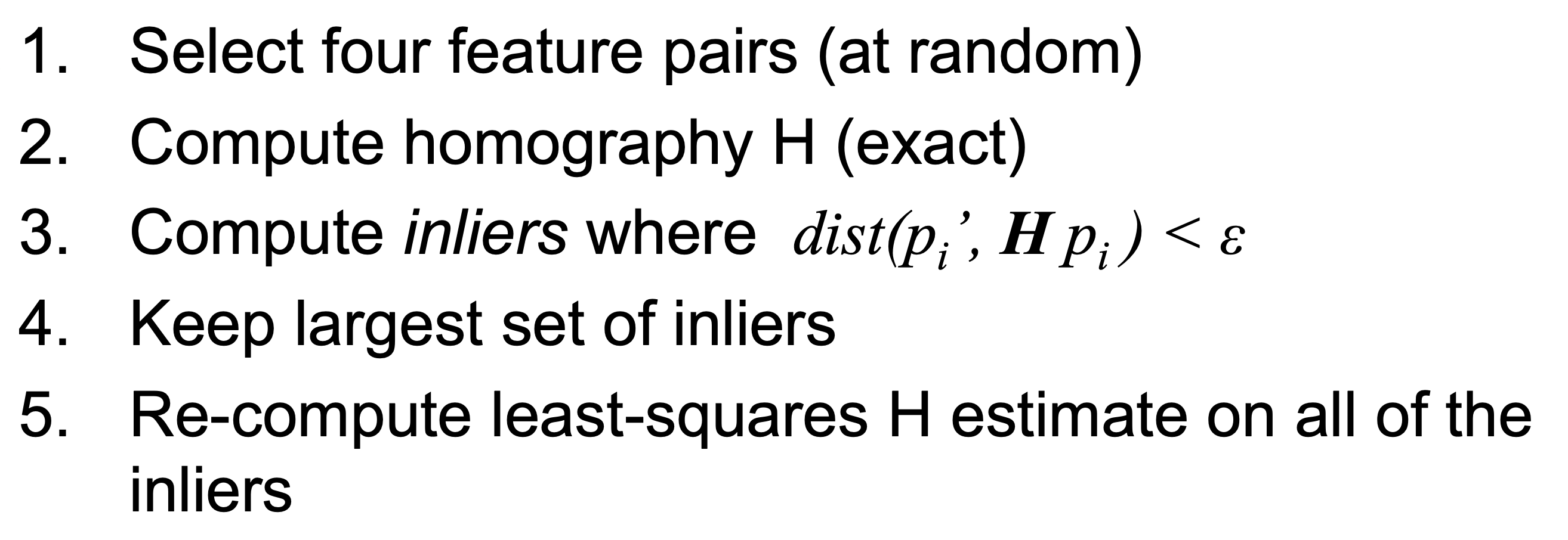
Steps 1-3 were repeated 10000 times with epsilon set to 1. In step 2, a least squares estimate of the homography was still used as it gave better results, and occasionally the matrix for solving the exact system was singular.
The mosaics are created the same way as above, but with the homography computed using the new techniques. The most notable difference in the first mosaic is the clarity of the tree and lamp post; in the second is the clarity of the books and chairs; in the third is the clarity of table to the left.
|
|
|
|
|
|
|
I learned how to stitch and blend images. The coolest thing was how well the output of the combination of images looked, and how rectifying can allow you to see parts of your image even better than in the original image. As well, learning to automate the process of choosing keypoints and achieving even better mosaics was very interesting.