Overview

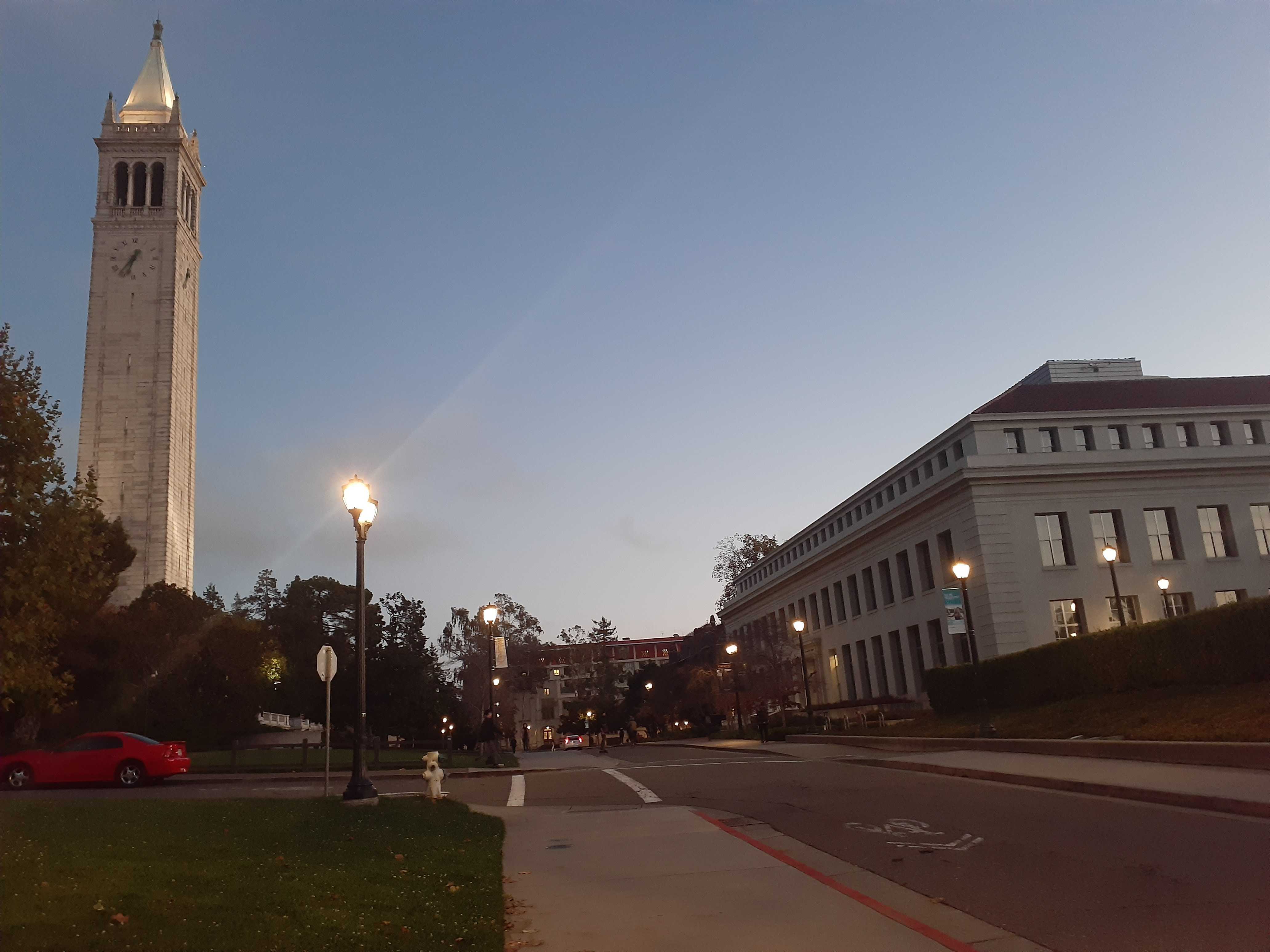
In this project, I first collected my own data such that the photographs contained projective transformations between them (same center of projection but different viewing directions). Afterwards, using these images, I recovered the homographic transformation between the images and used the homography matrix to warp and rectify the images. Finally, using my implementation, I was able to warp images onto a base image and blend them together to create a mosaic.

Recover Homographies

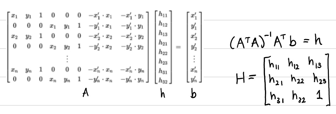
In order to recover the homography between two given images, I first had to use ginput to manually define the 1:1 correspondence points between the images. I specifically chose points on objects that were closer in terms of depth/more prominent in the picture, and had a distinct shape. I made sure to define more than 4 points for images that did not involve a primarily frontal-parallel plane, as our homography matrix has 8 unknowns and 4 points gives us exactly 8 values, leaving us with an unstable homography recovery. Thus, I collected more than 4 points to ensure an overdetermined system that I could solve with least squares. Here is the system that I used to recover the homography:

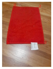
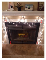
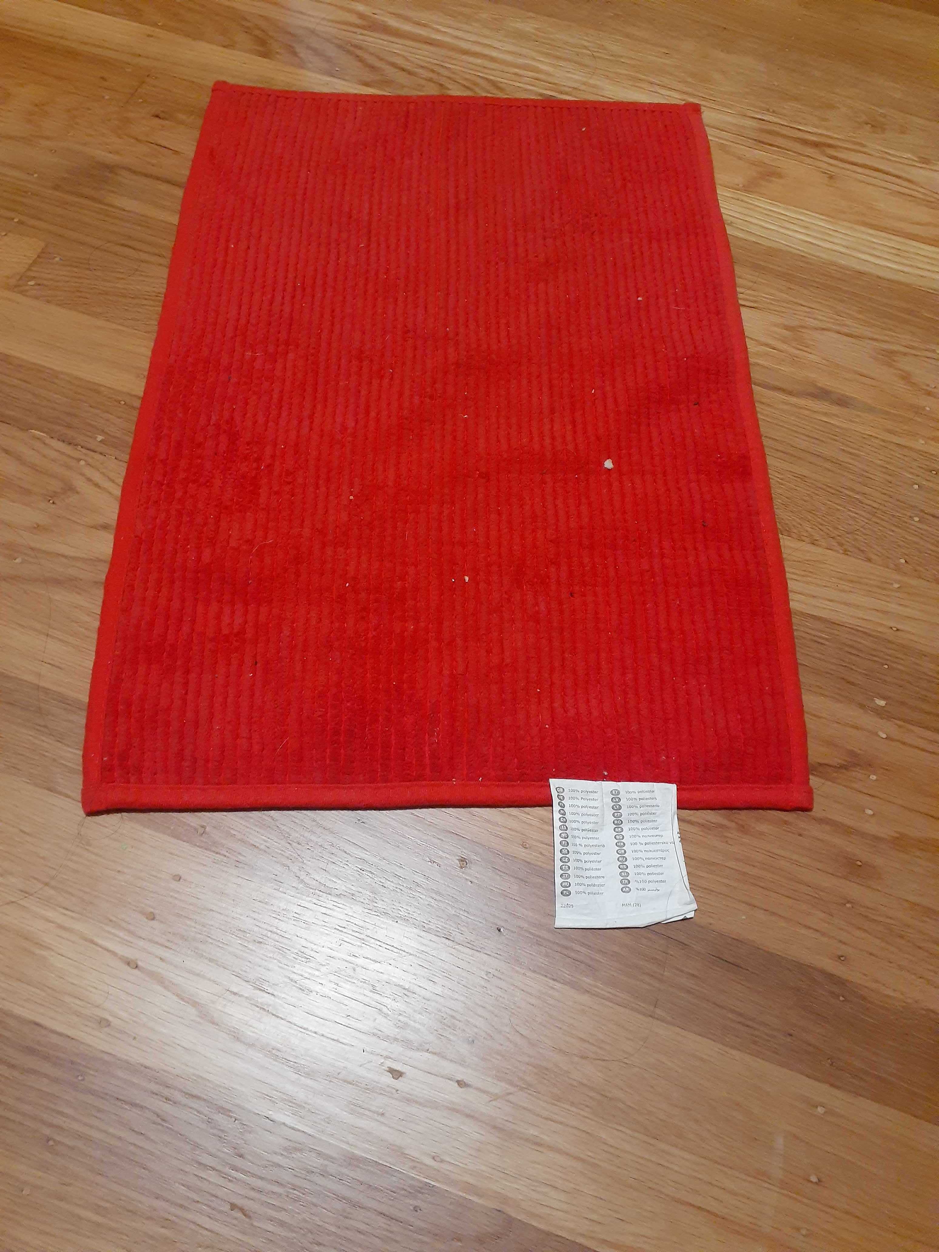
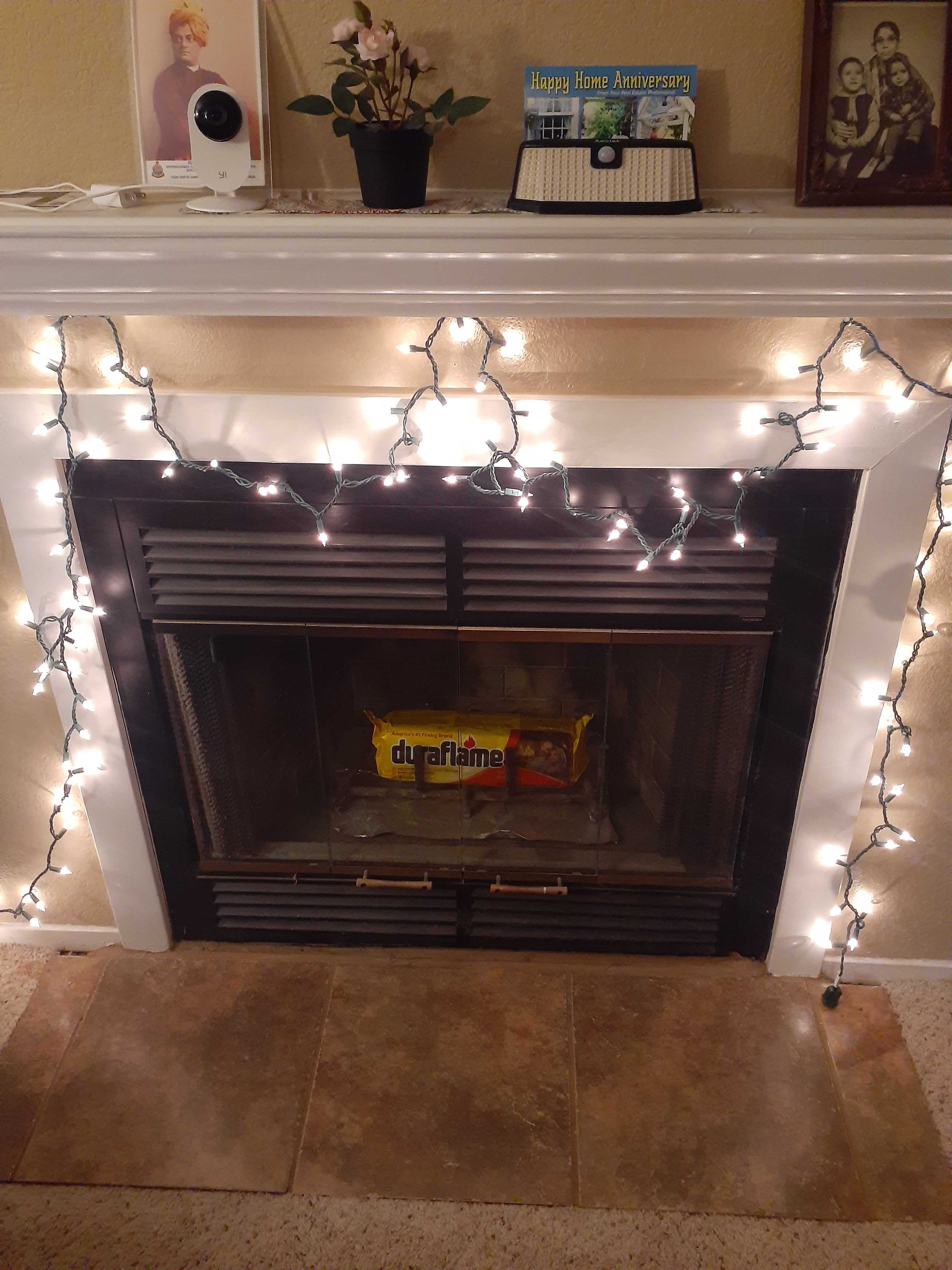
Here are some examples of the frontal-parallel correspondence points I used:

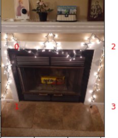
Warp the Images + Image Rectification

After constructing the homography matrix H using least squares, we can either use forward or inverse warping to rectify the image. In my case, I used inverse warping by defining the coordinates of the output image and passing them into cv2.remap() in order to "look up" where every destination/output pixel maps to in the original image. In order to define the output coordinates, I had to find the bounds of my output image, which I did by using the homography matrix to transform the input image corners into their transformed coordinates and finding the minimum and maximum of their corresponding x and y values.
In order to test both my homography recovery and warping function, I used the above images and their correspondence points to rectify the images. Here are the results:

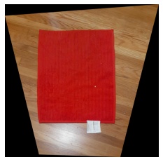
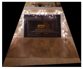
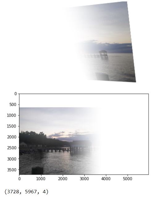
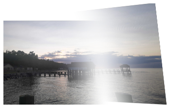
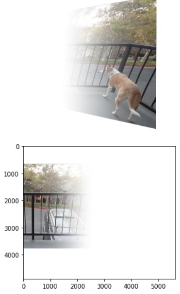
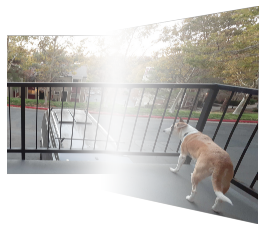
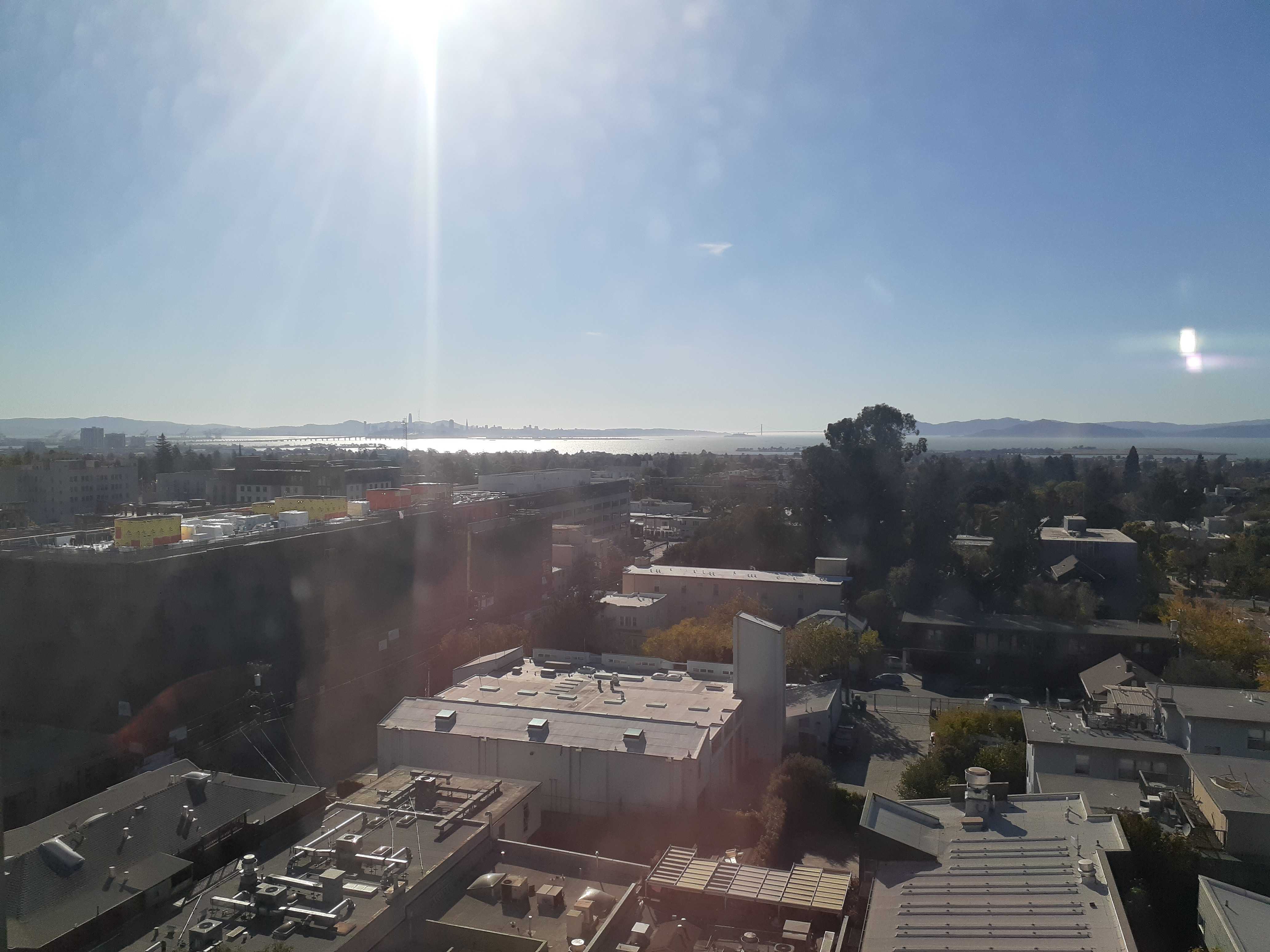
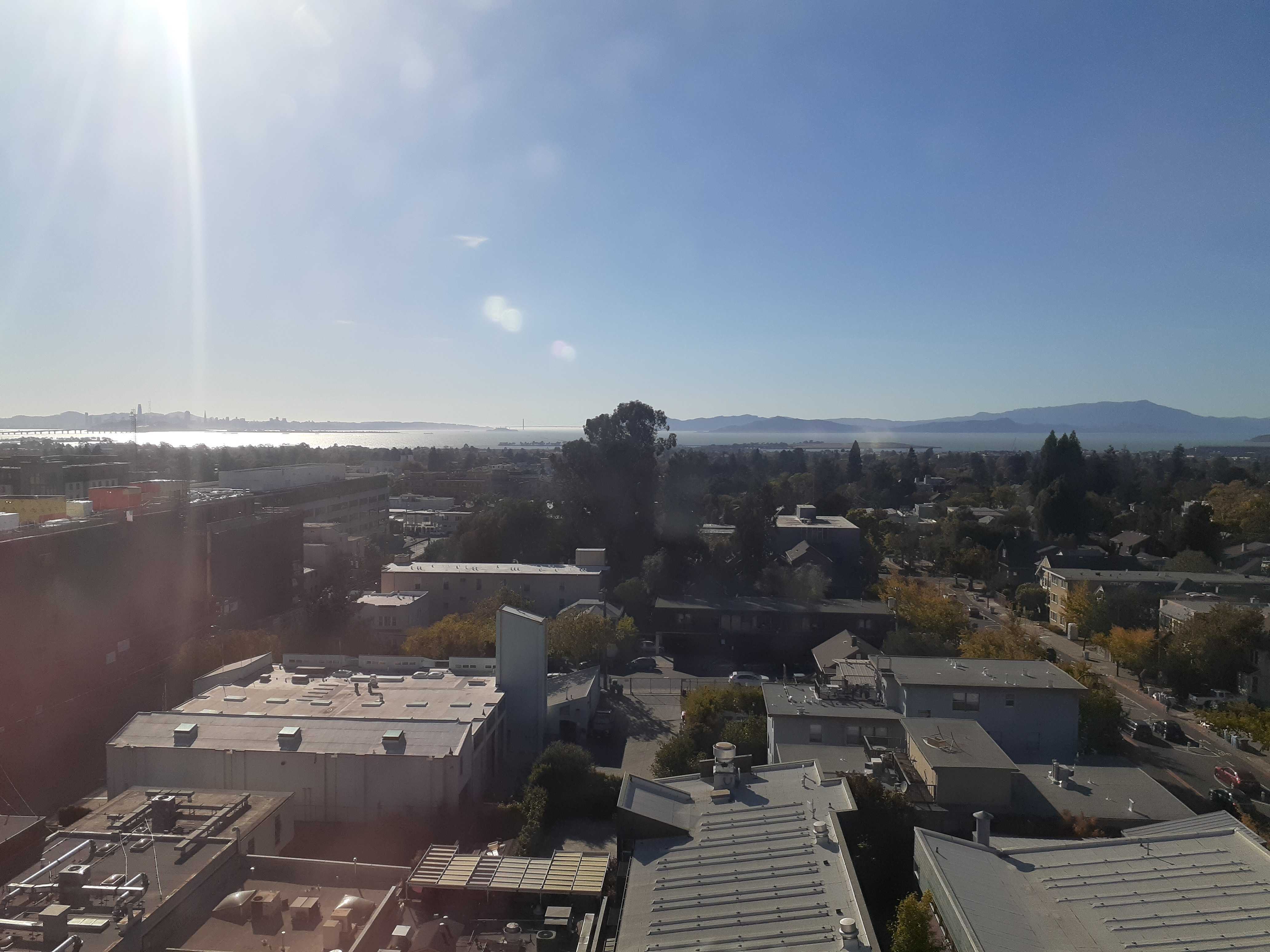
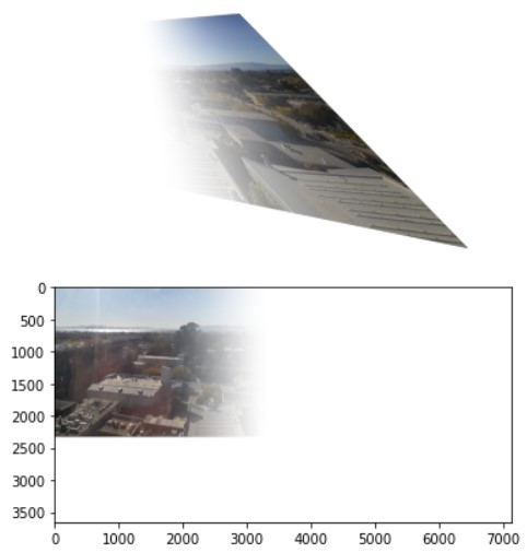
Blend the Images Into a Mosaic

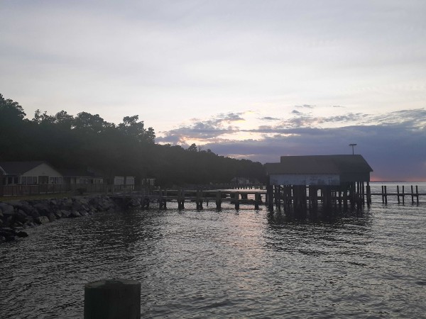
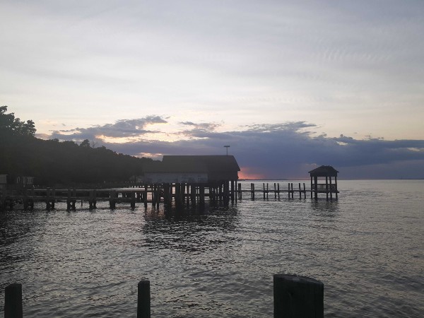
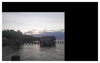
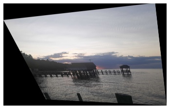
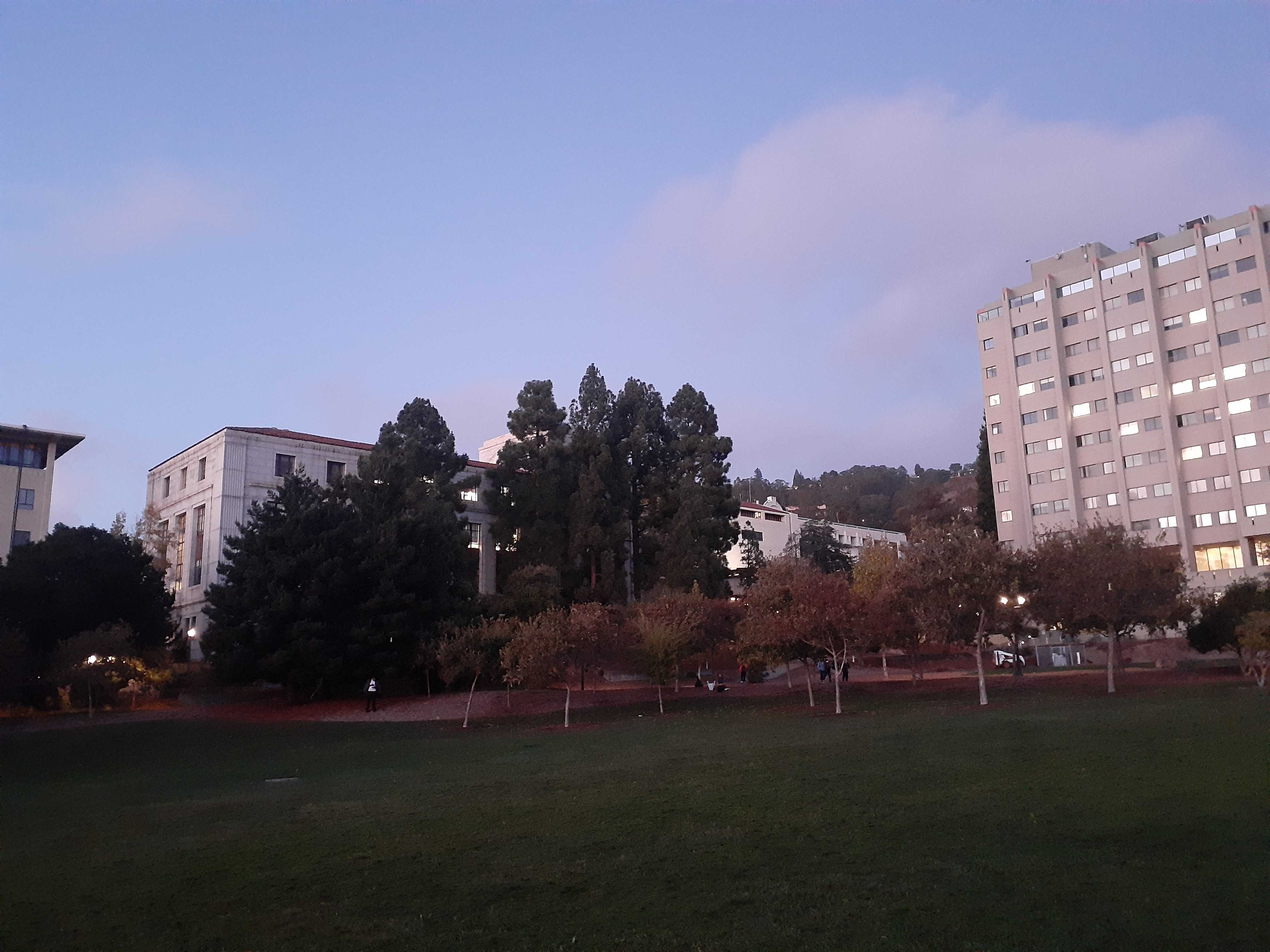
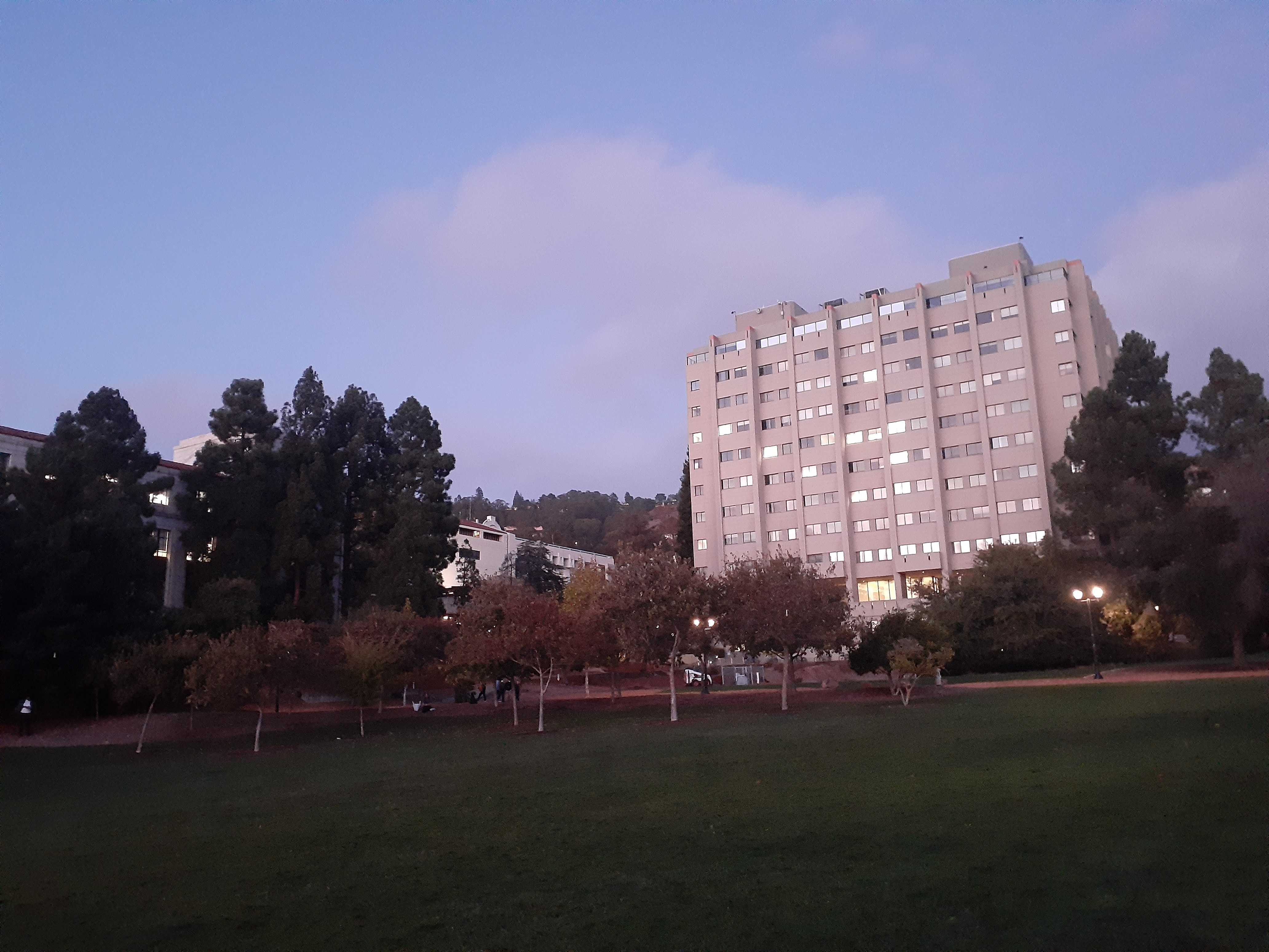
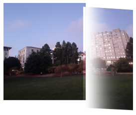
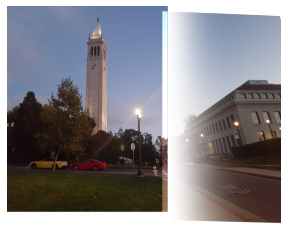
In this part of the project, I utilized the homography recovery, output image bound calculation, and inverse warping functions to create a mosaic out of a set of images. I set one of the images as my "base image" and warped the other images to it. In order to blend the images together, I created an alpha channel and used weighted averaging. Here are three mosaics using the above methods:

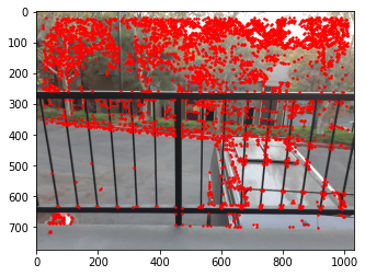
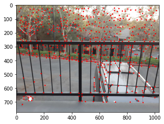
Detecting Corner Features in an Image

In this part of the project, I utilized the Harris Corner detector in order to detect the corners within the given image. I could adjust the threshold which modifies the minimum peak intensity and thus is more stringent on which corner points are selected. In the following images, a threshold of 0.1 is used:

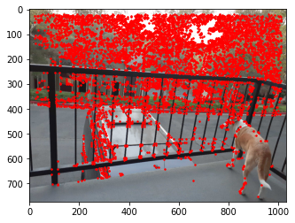
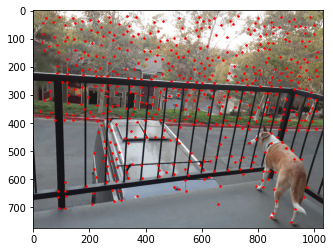
I also implemented Adaptive Non-Maximal Suppression (ANMS), which involves using the corner strength of each of the pixels and computing the minimum suppression radius, allowing us to only choose points that are spatially well distributed throughout the image. Hence, we only make sure that we only pick points within the same neighborhood if they are very strong corners.:

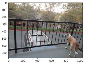
Feature Descriptor Extraction + Matching

In order to match the corners detected between two images, so that we can later compute the homography, we first need to extract a feature descriptor for each of the corners. We can do this by sampling 40 points around a corner point detected from Harris + ANMS, blurring it using a Gaussian kernel, and then downsampling it to an 8x8 patch. Afterwards, we compute the SSD between each feature descriptor pair between the two images and find the first and second nearest neighbor. Using Lowe's Trick, we can then compute the ratio between the SSD of 1-NN and 2-NN and only accept that corner as a match if the 1-NN is significantly better than the 2-NN's SSD, hence bounding it by a threshold. The following are the feature matches as a result of the above algorithm:

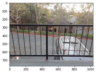
After using Lowe's Trick to narrow down our matches, I implement 4-point RANSAC in order to ensure that all matched points are "inliers"/definitely a true match between the two images. We can do this by randomly selecting 4 matches outputted from Lowe's, computing the exact homography, and checking whether or not the squared distance between the warped points outputted from applying the homography to one image's points and the true corresponding points in the other image is bounded within a certain threshold, calling them "inliers". We find the largest set of inliers and use those to compute a more accurate homography via an overdetermined system. The following are our matches after running RANSAC:

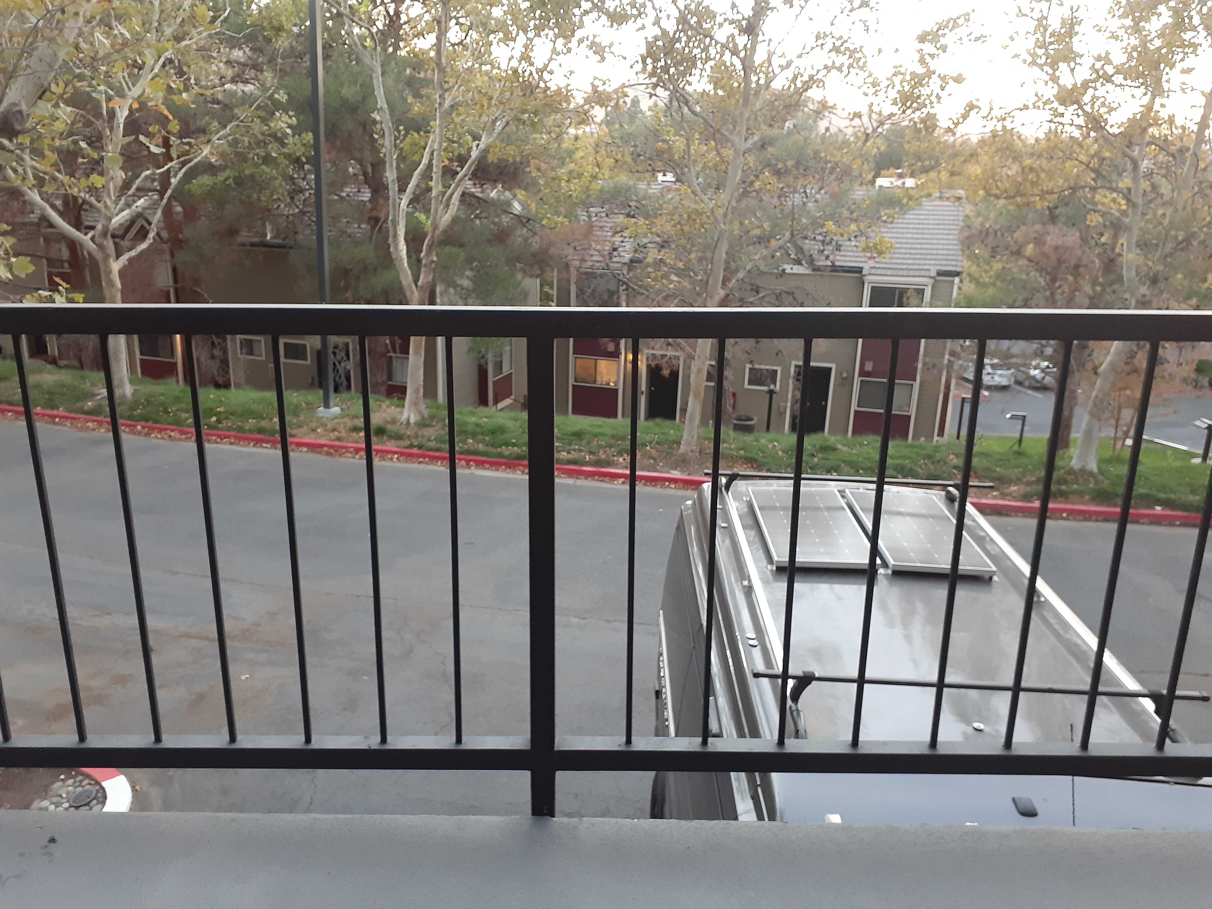
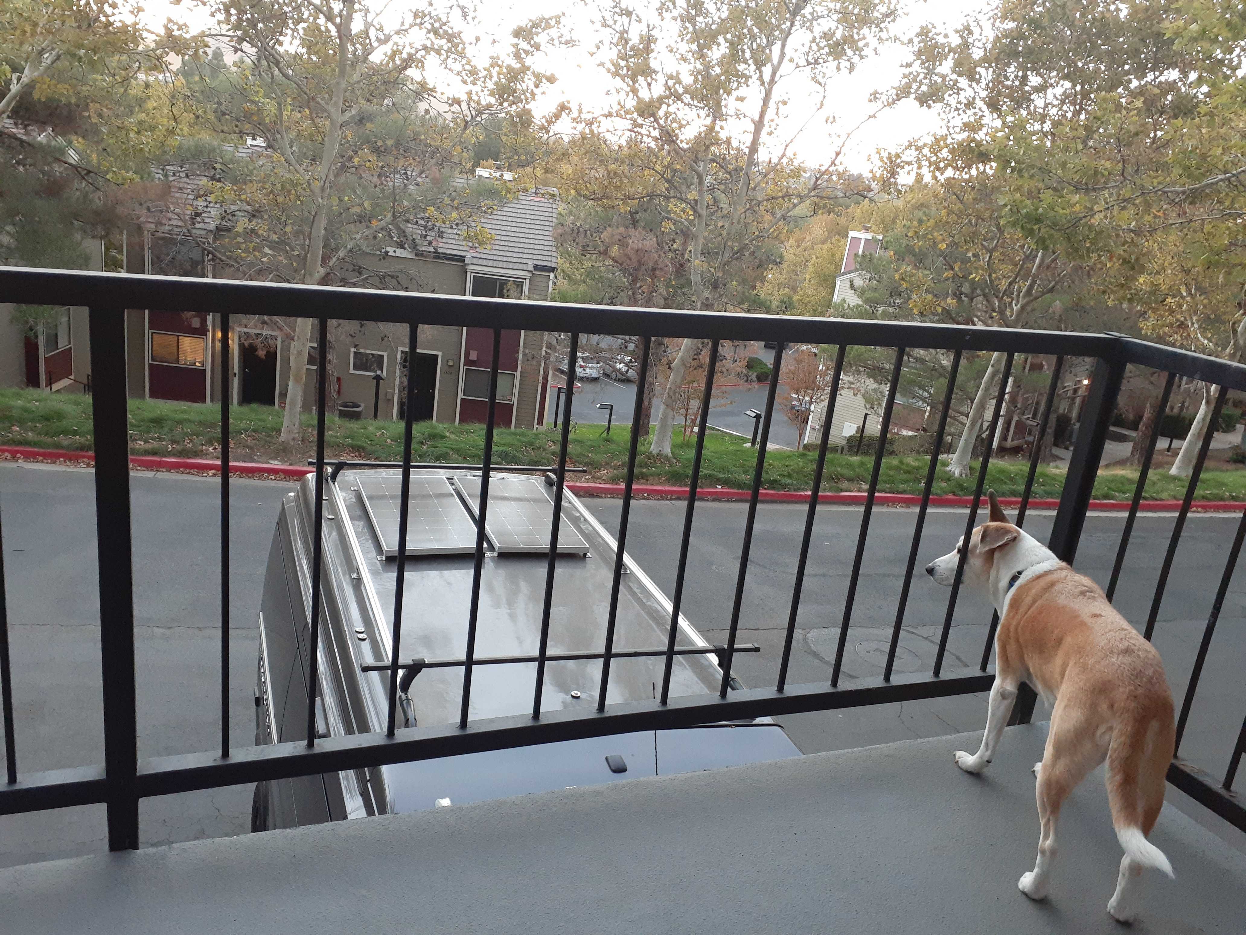
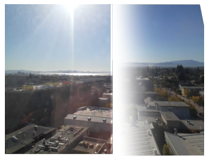
Part B: Blending our Images into a Mosaic

In this part of the project, I utilize the same algorithm I used in Part A to stitch my images together-- now using the homography outputted by RANSAC instead. I set one of the images as my "base image" and warped the other images to it. In order to blend the images together, I created an alpha channel and used weighted averaging. Here are three mosaics using the above methods. My alpha blending is a bit bugging, carrying on from Part A:

What I learned!

I learned a lot doing this project, from learning how to recover homographies from just a few points to realizing how applicable inverse warping is to so many cool applications. Additionally, in part B, I learned how much more efficient and effective automatically detecting points within images is, and how this can truly allow our stitching process to scale.