Overview
In this project, I create a mosiac from multiple images to a base image. I also rectify images to make them straight up. This involves creating homographies and converting between them.
Shooting the Pictures
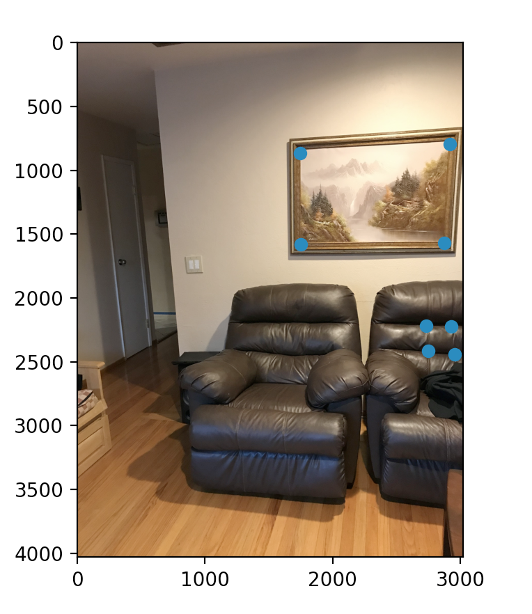
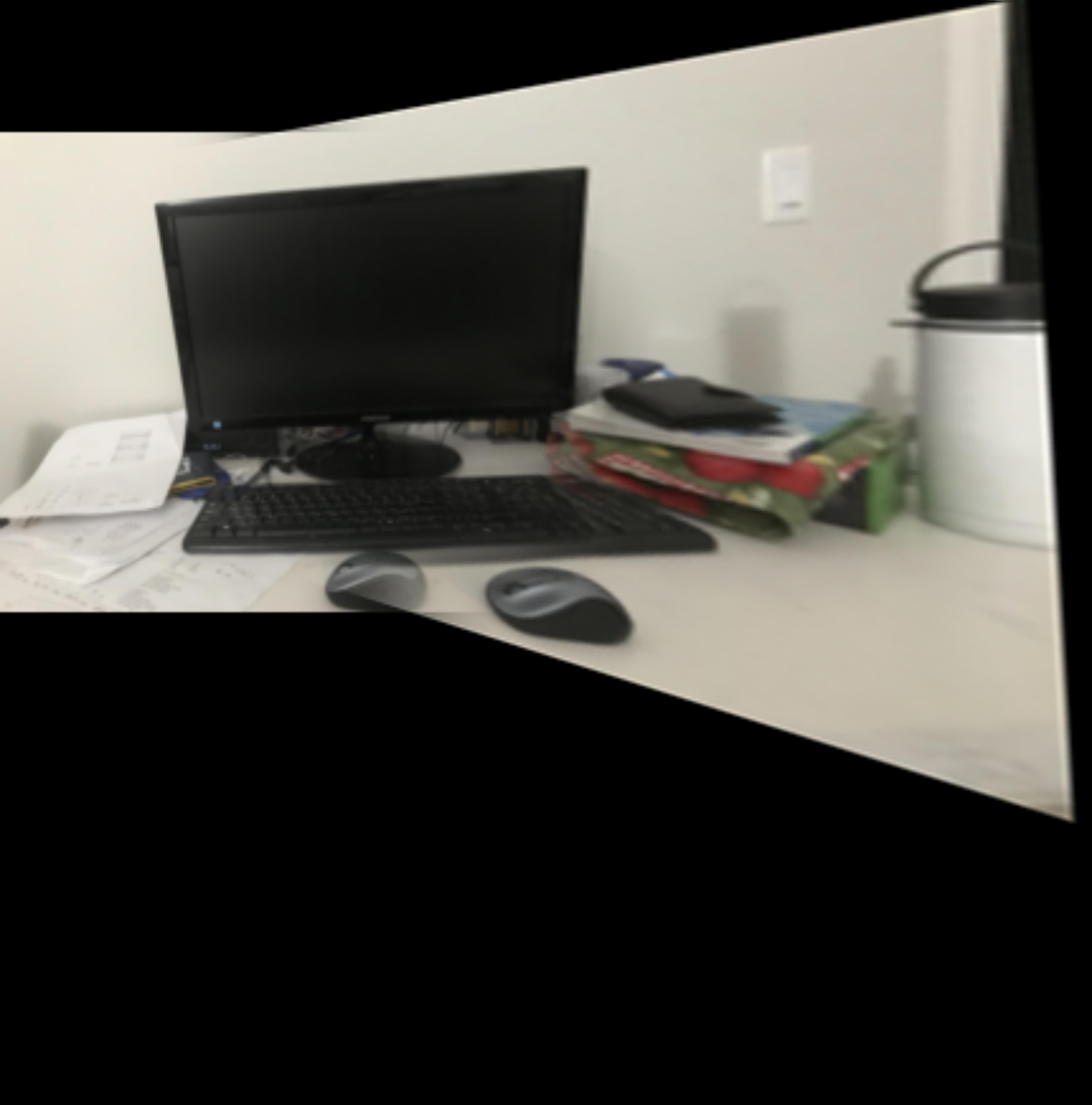
To define correspondences between two images, I selected easy to see points in the following 2 images. All these images describe a single plane.
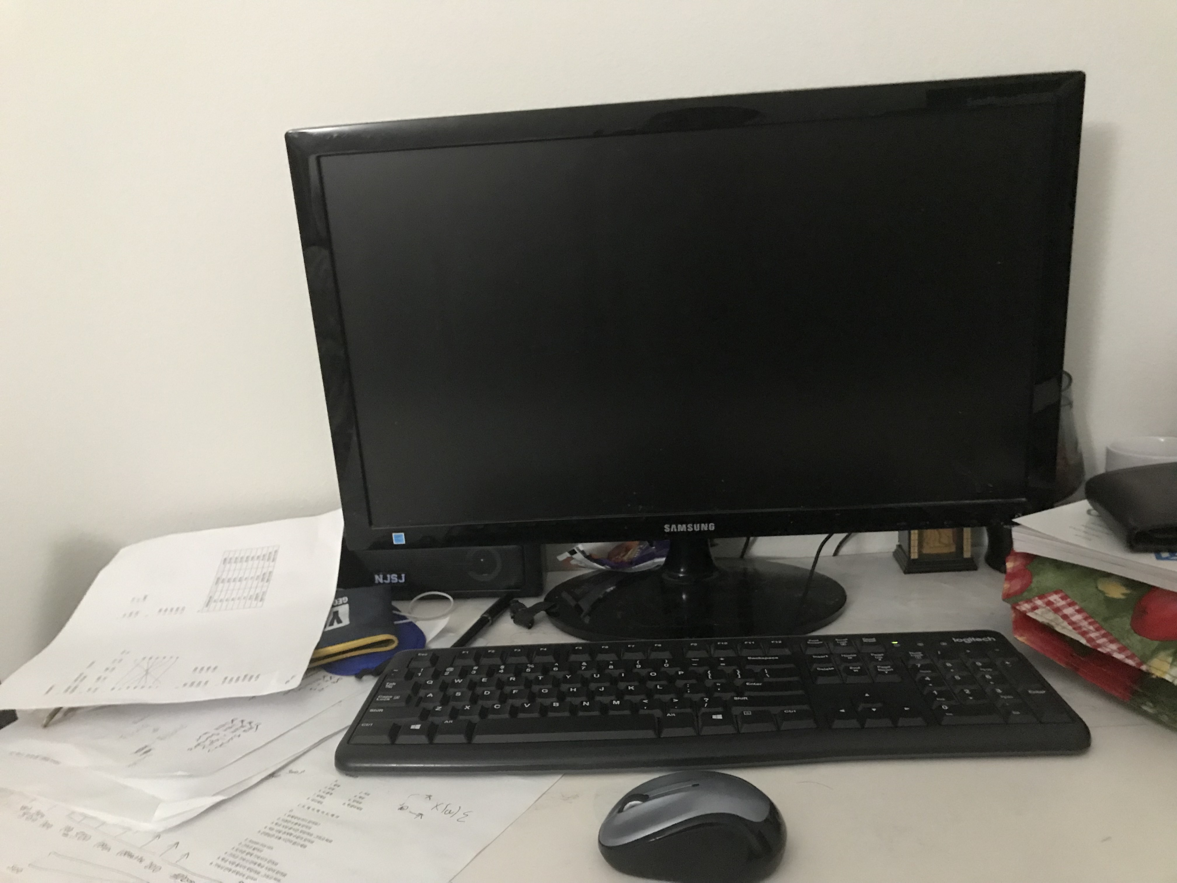 Laptop image left side. With the inside monitor being the four coordinates chosen
|
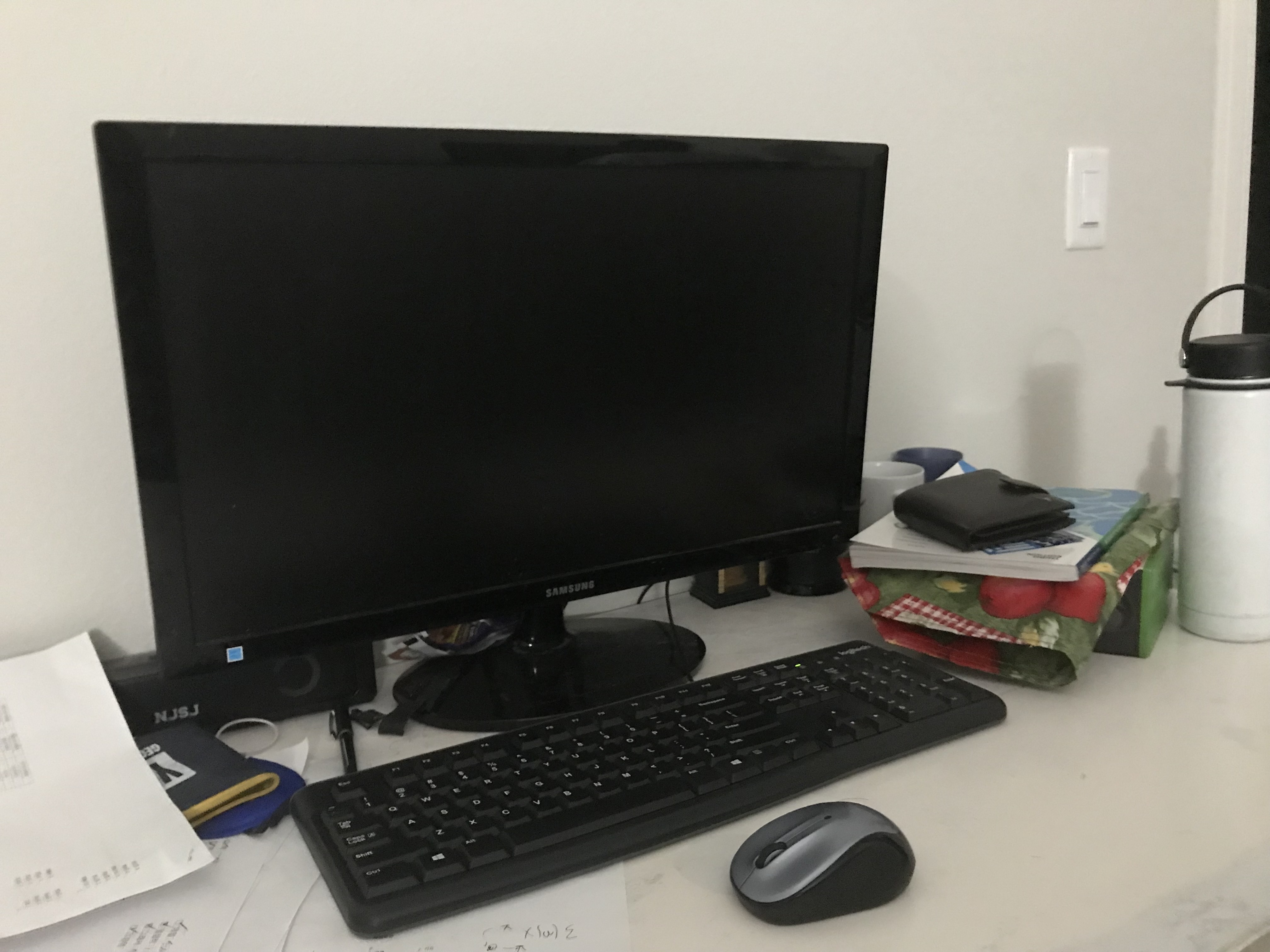 Laptop right. With the inside monitor being the four coordinates chosen
|
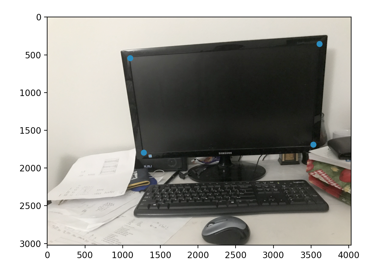 Laptop image left side. With the inside monitor being the four coordinates chosen
|
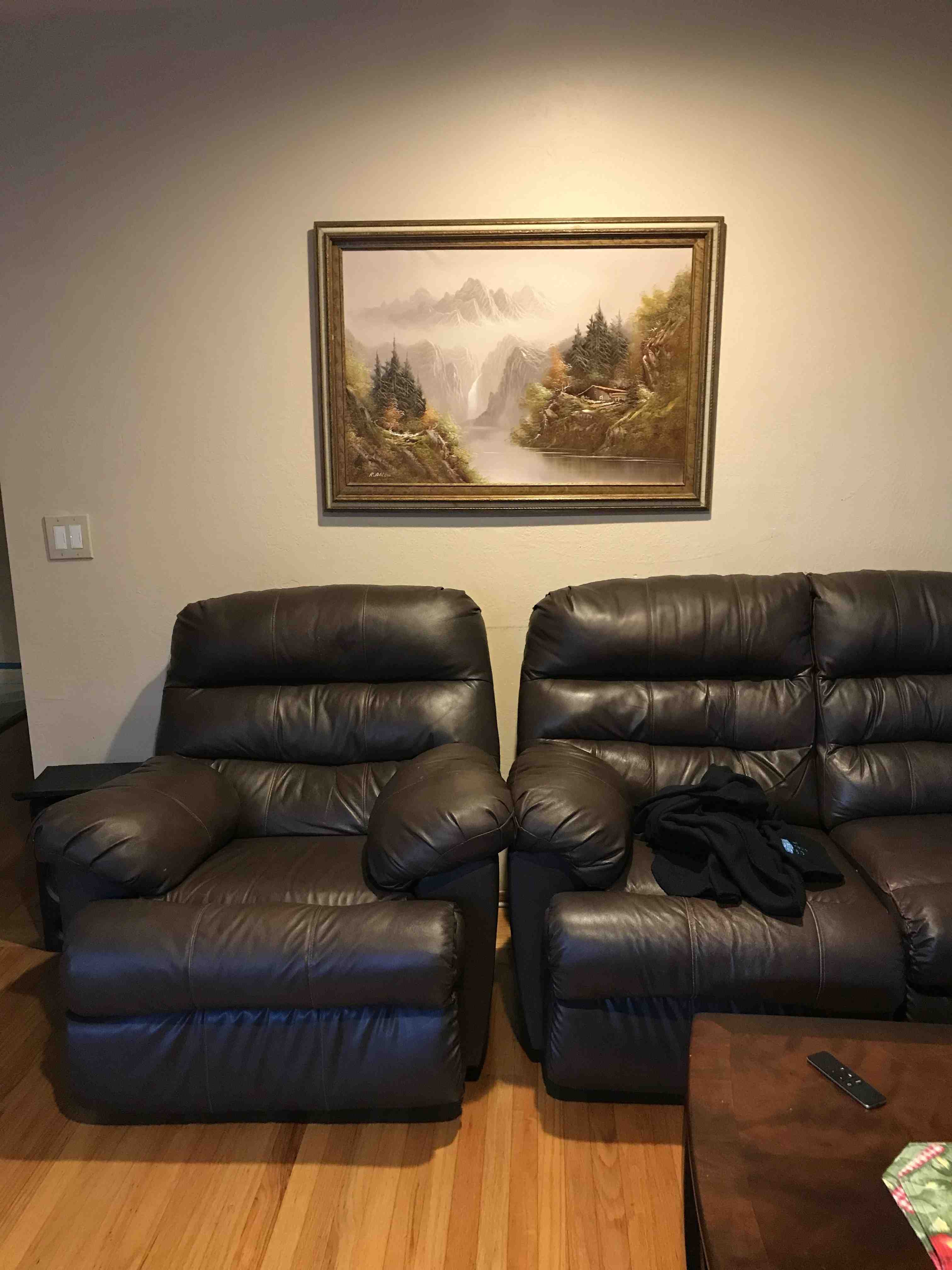
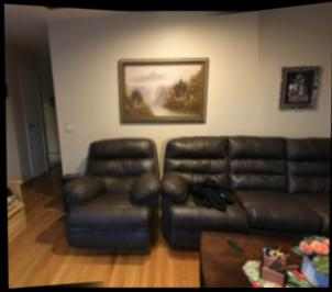
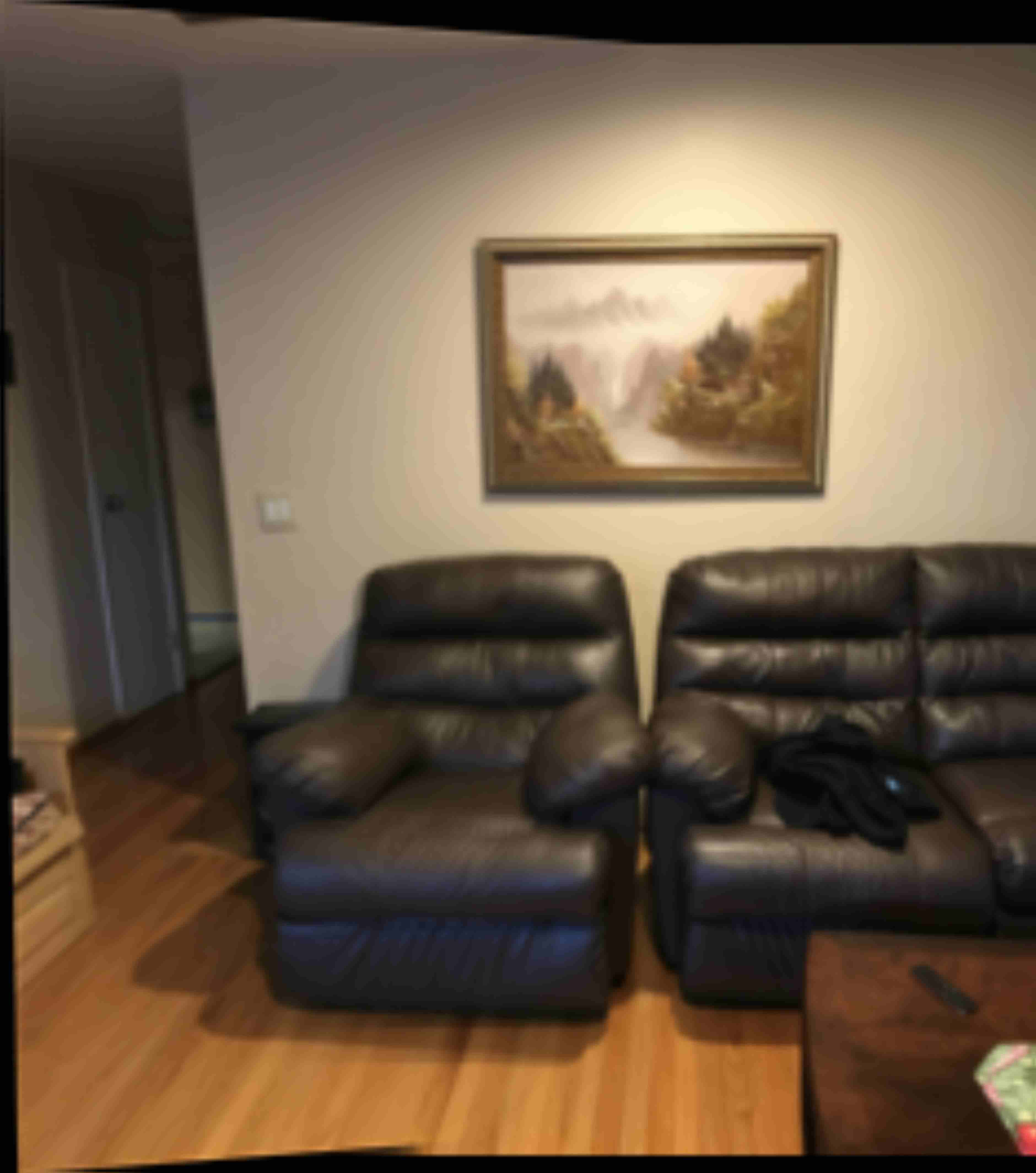
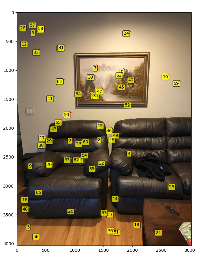
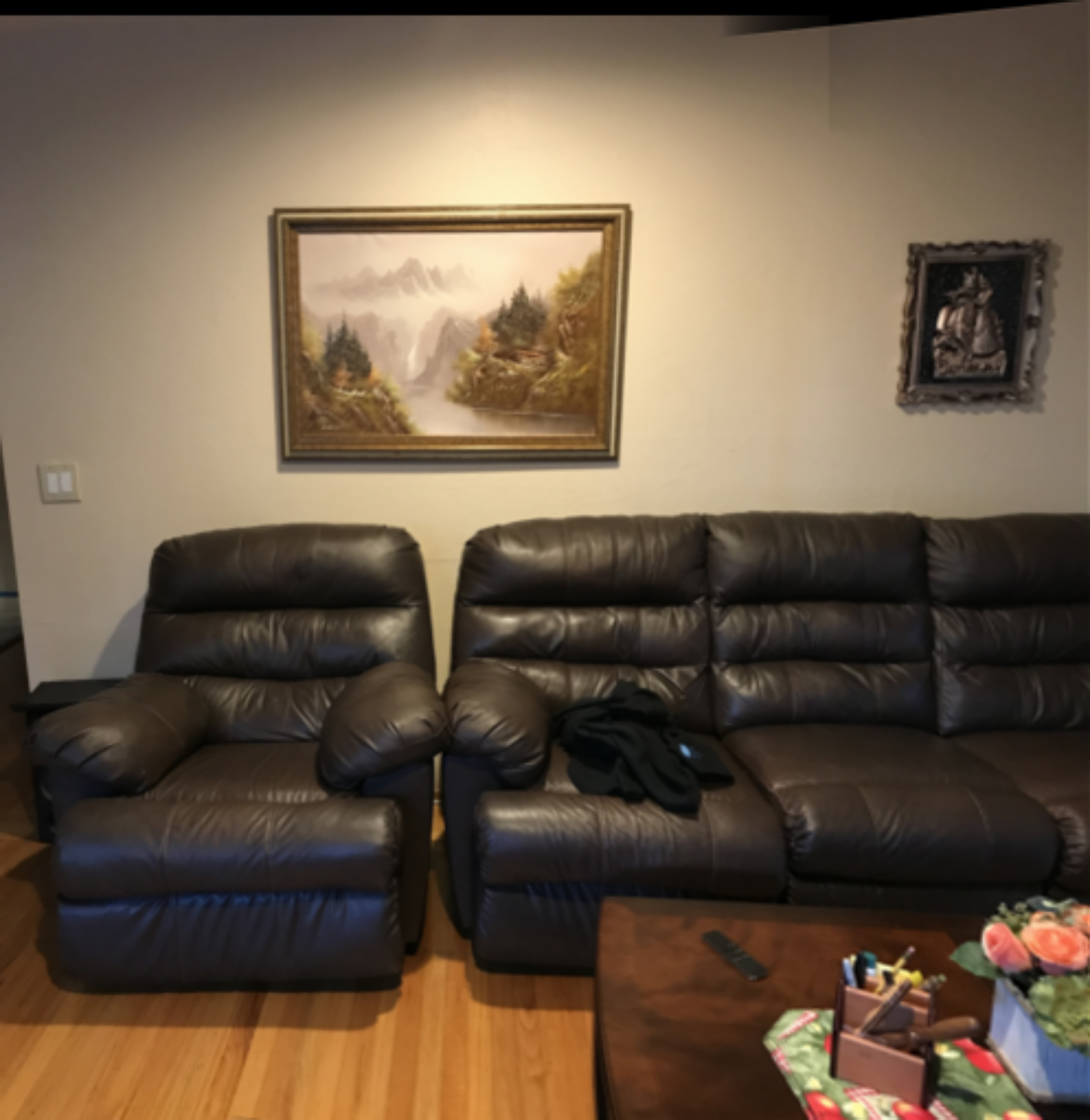
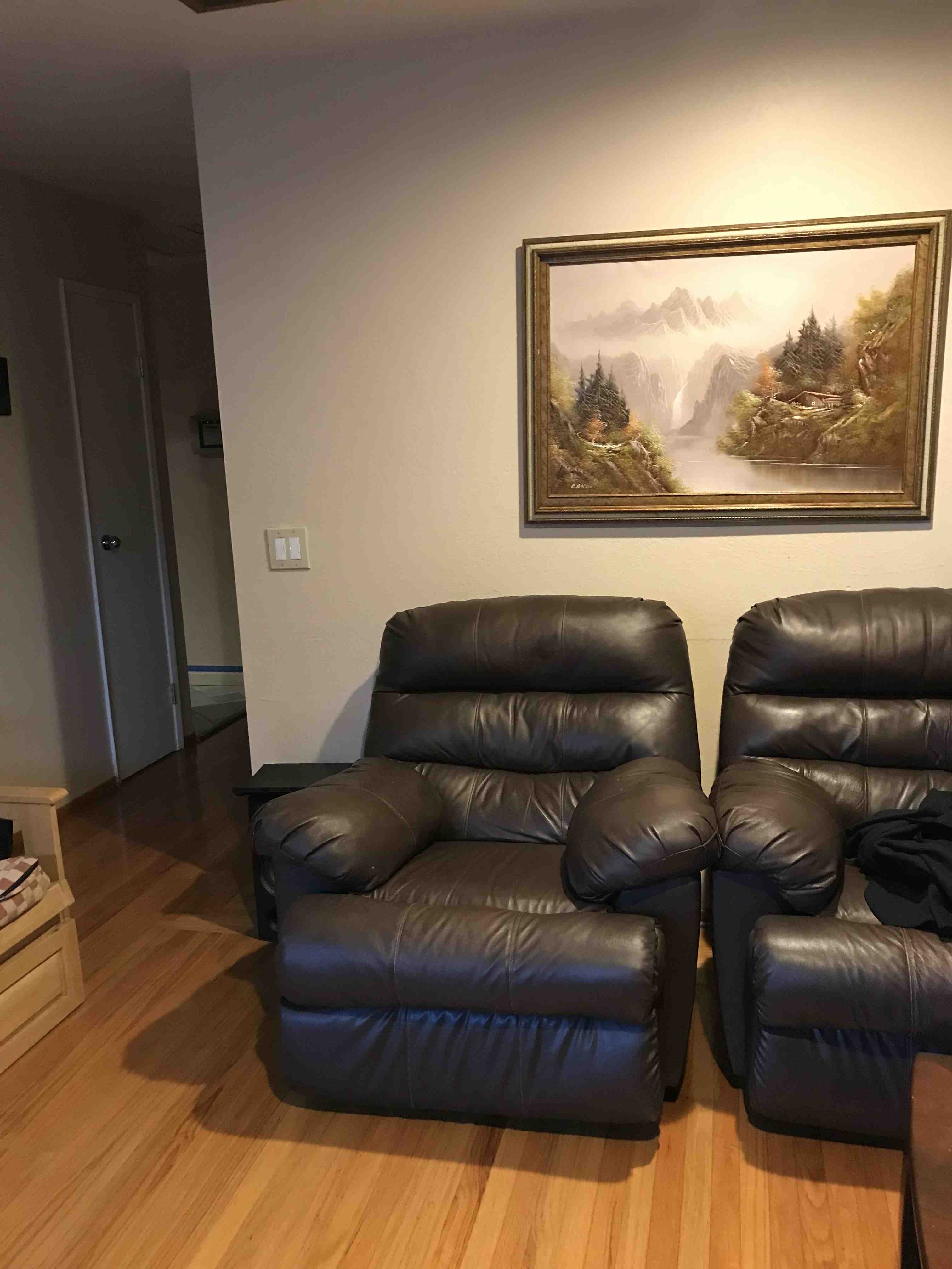 left chair with painting and chair as points
|
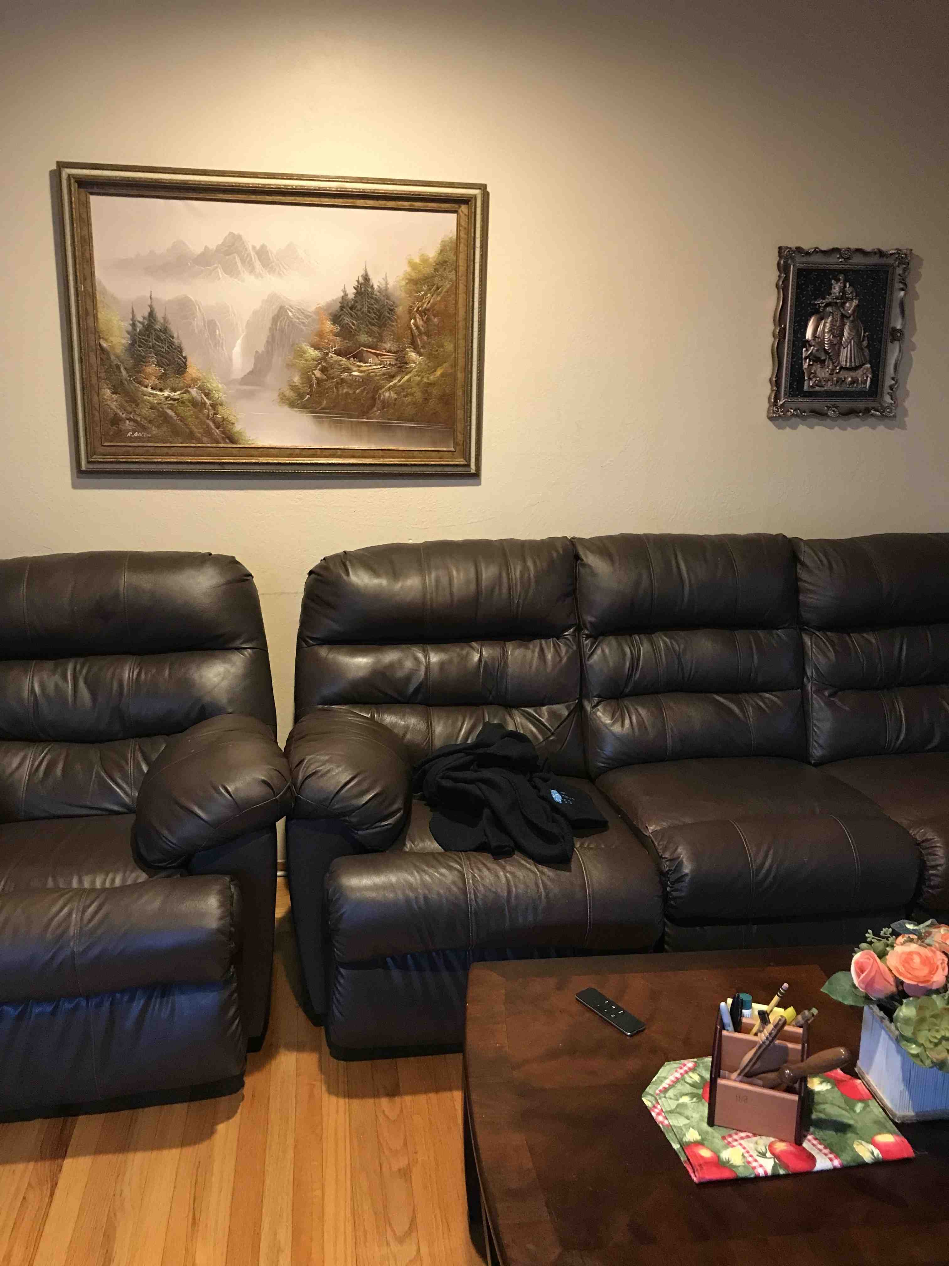
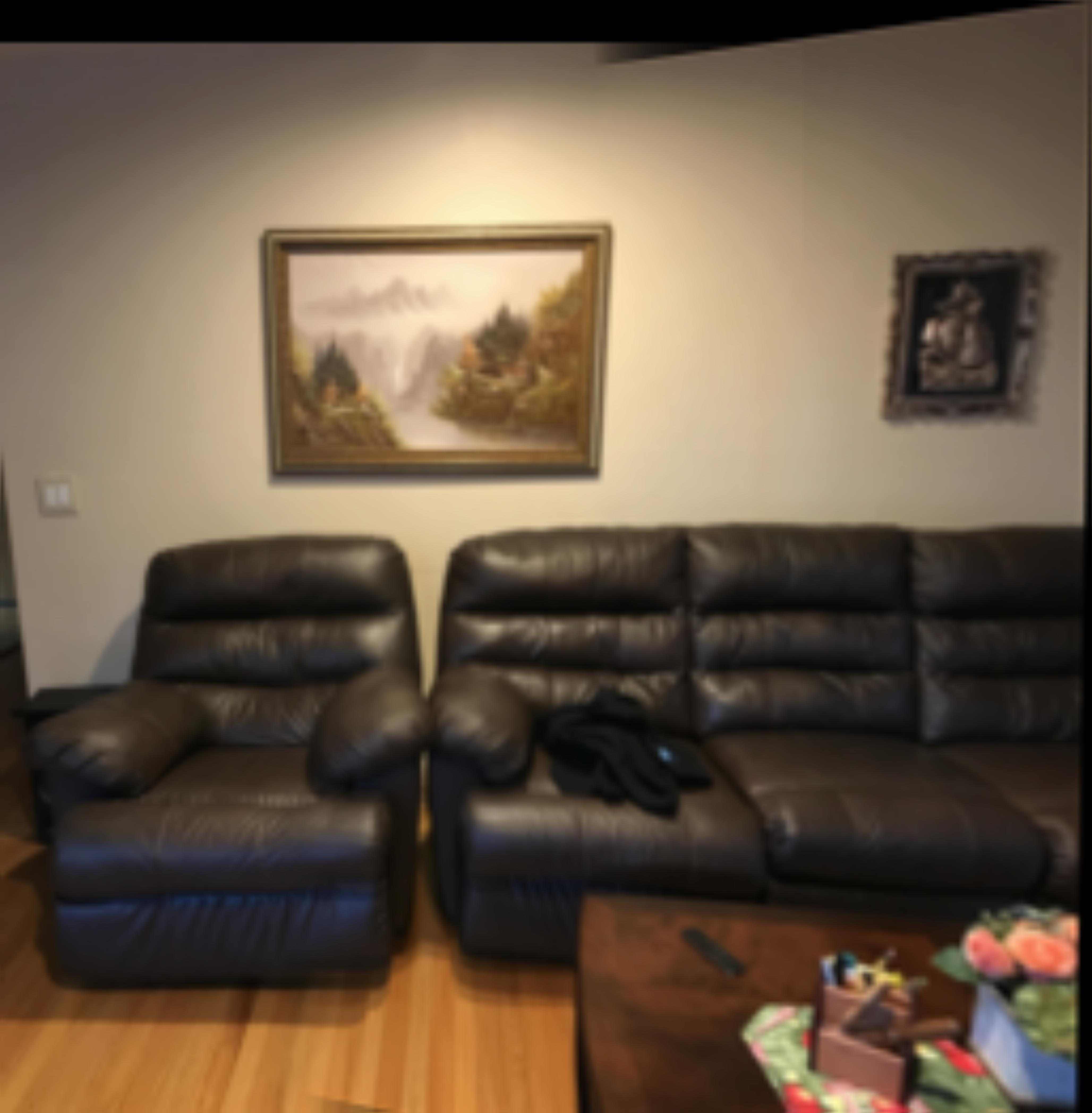
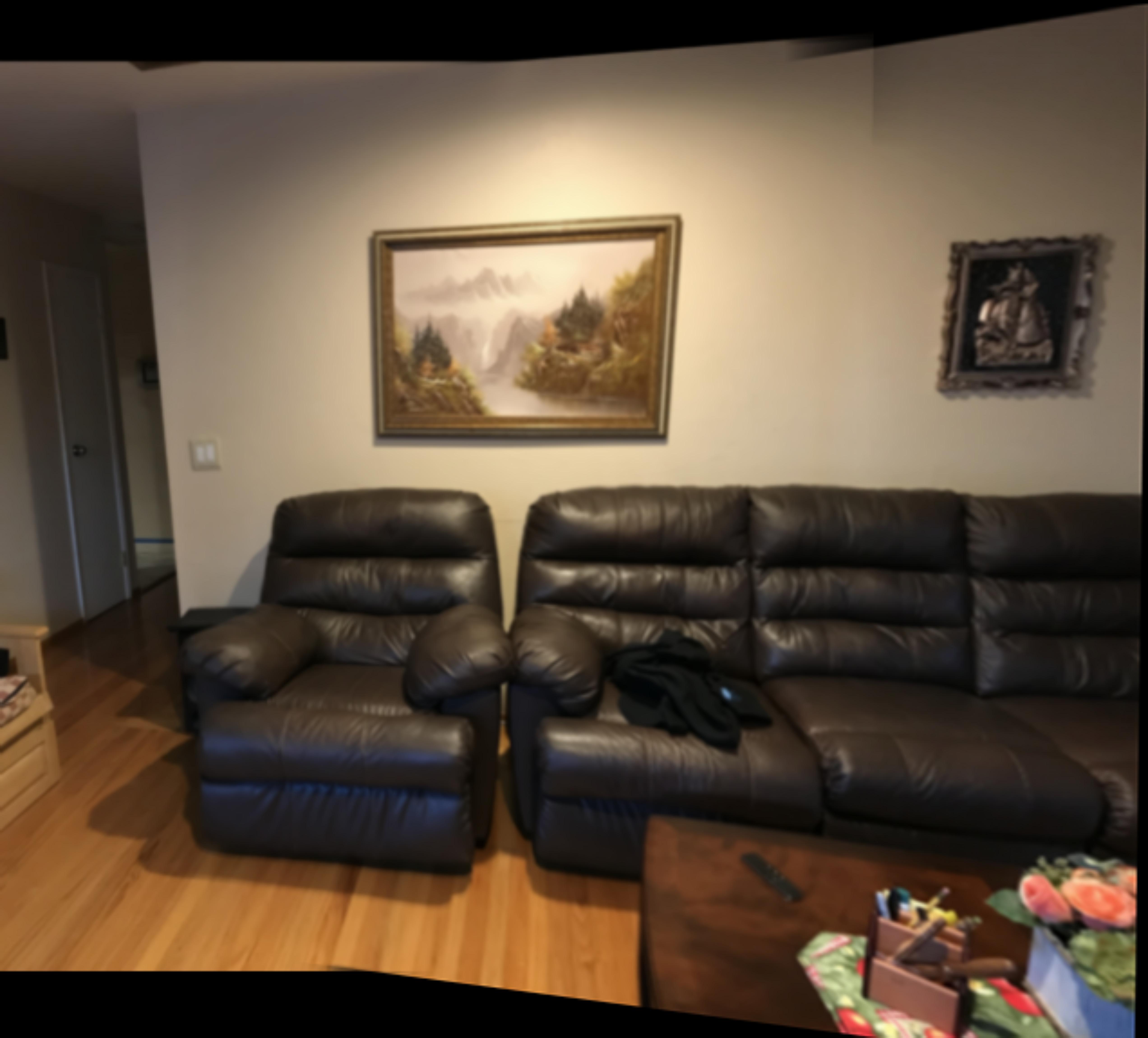
 center chair with painting and chair as points
|
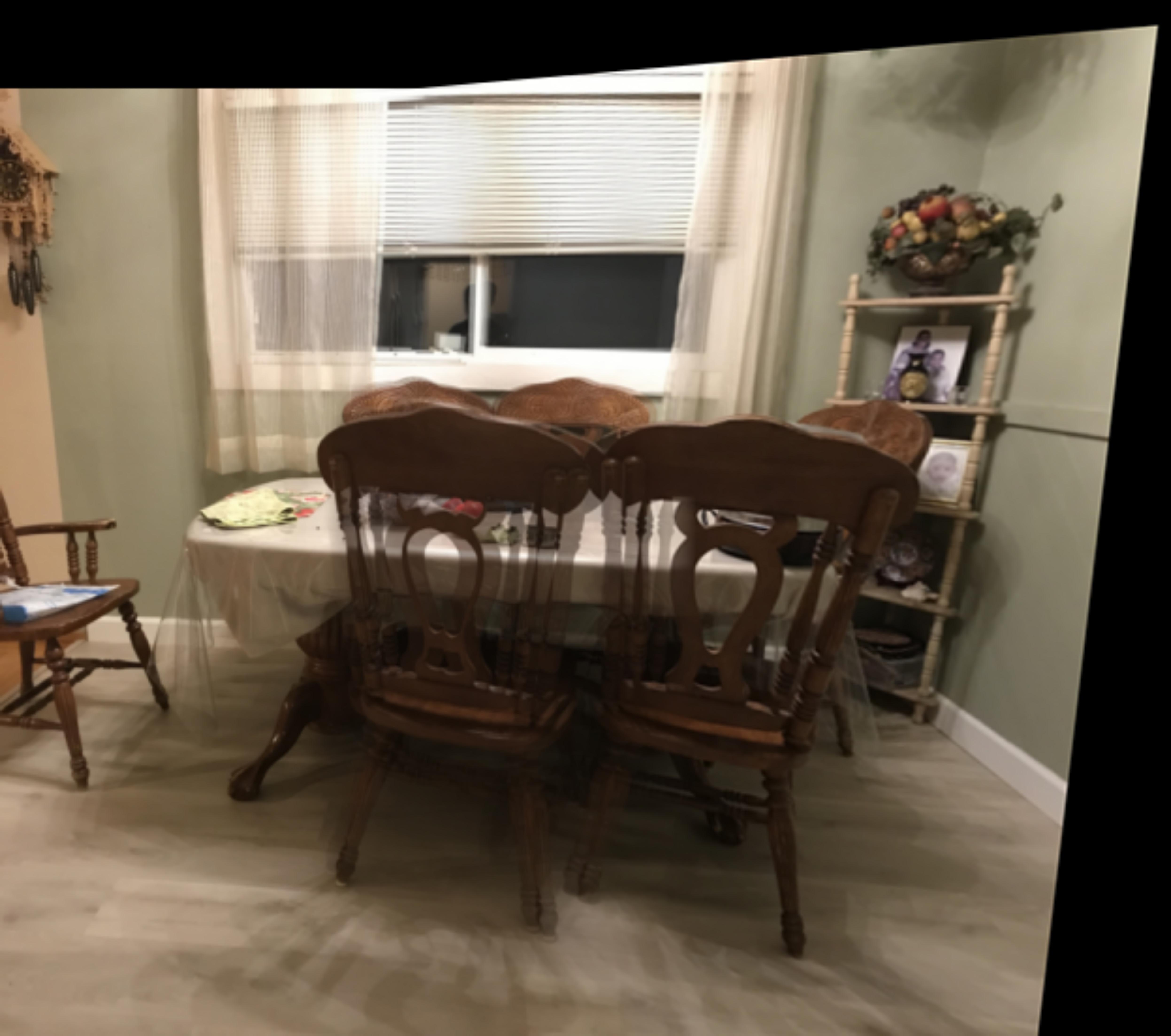
 right chair with painting and chair as points
|
 left chair with painting and chair as points
|
Recovering Homography
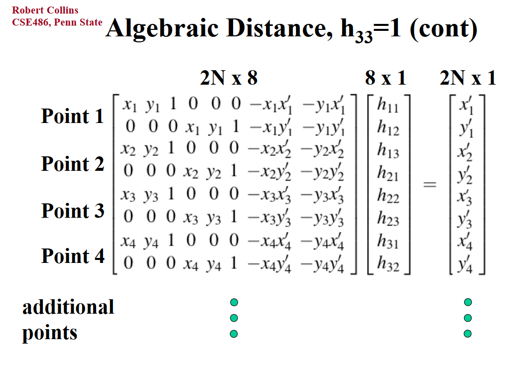
In order to recover the homography, I took the points from the two images and then computed the homographic transform.
The regular homographic transform between two sets of points is
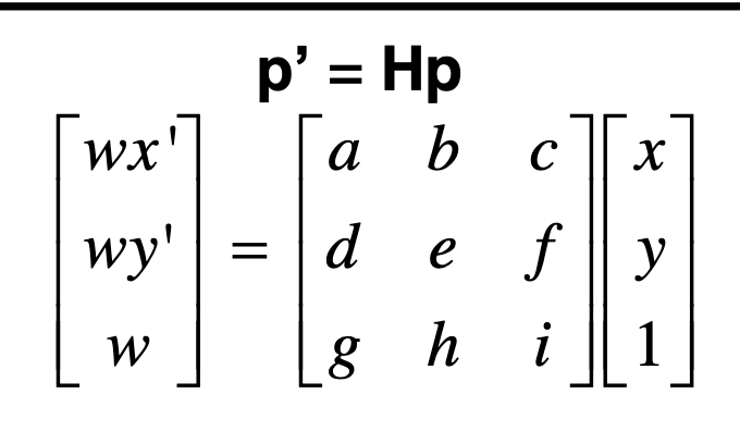 Homography Image
|
By setting the scale paramater i to 1, we can get the the equations (w = gx + hy + i). Plugging this into the other matrix, we getting the following larger matrix,
I created the following grid:
 Homography Image
|
We find this grid by setting the scale factor to 1 and unrolling the homographic transformation matrix in lecture.
This grid represents a transformation from image1's space to image2's space. This transformation is non affine. I generalized this code to accept arbitary number of x and y points. This made an overconstrained matrix that can be solved via least squares approximation.
Warping the Images
In order to warp the images, first the mosiac border needs to be computed. This can be computed by computing by computing the homography of the corners of the image. This is then put into the new larger space. This space might be bigger than the space of our images, so we need to adjust the size to be max(transformation) - min(transformation). Since we might have negative values after transformation(less than 0), we can compute a affine translation to make it so that points are algined with the new size.
With the translation, we can apply an affine transformation on the homography matrix to have it return values in the right order. I also compute the inverse to go from this homography space back to the original space.
To get the points in the new space, I create a meshgrid of all the points and apply the homography. Then, I remap them them cubic interpolation into the true mosiac's size.
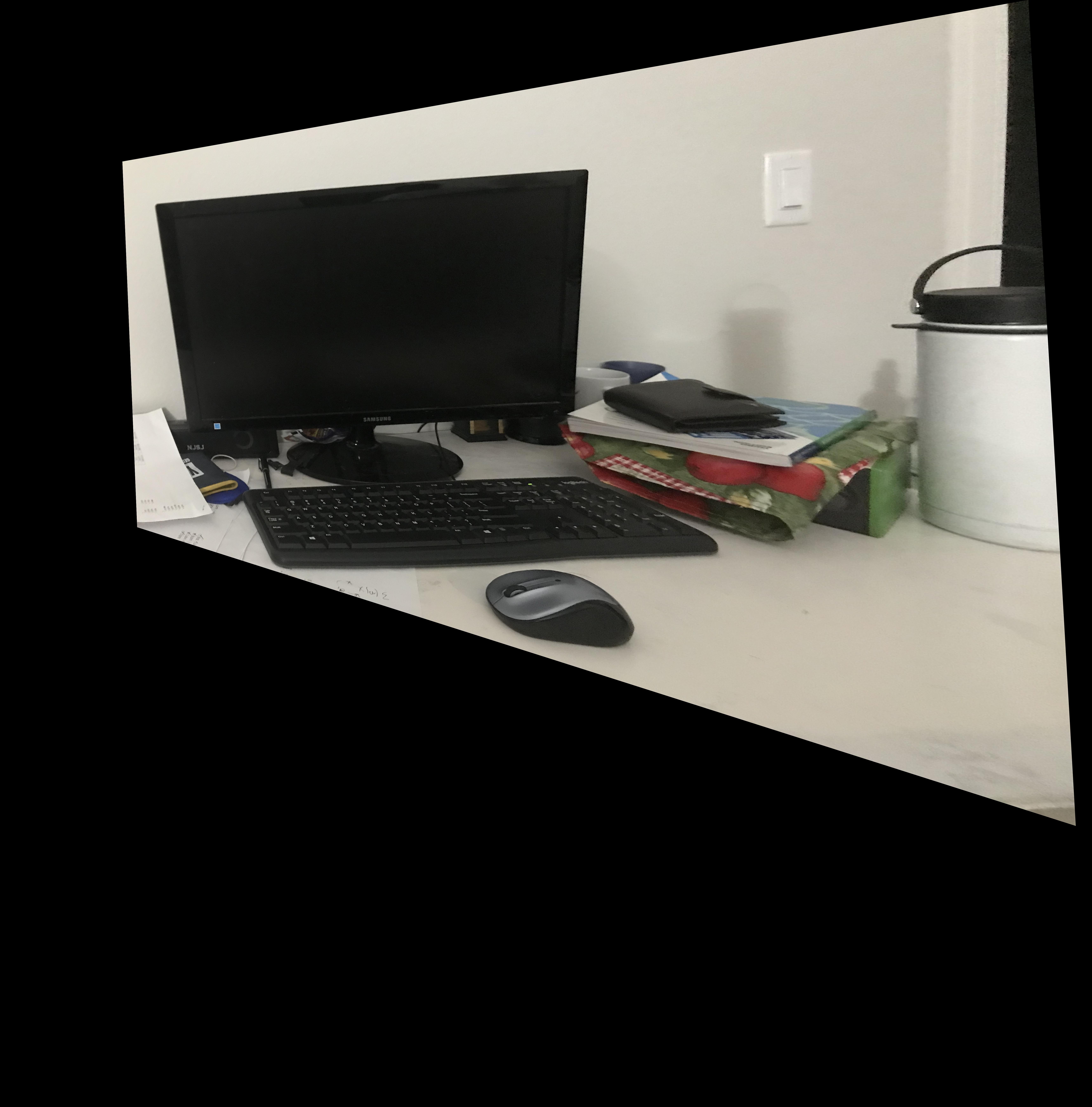 Just one warp of the image
|
Rectify Image
Rectifying the image was very similar to the warping of the image. This time, after the 4 points were selected, we computed a the leftmost corner and rightmost corner. We can then compute a rectangle using those four points.
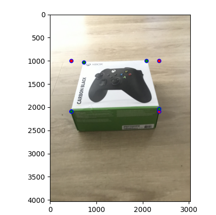 The red points are the new coordinates added to rectify.
|
.
Then, this can be run through the warping code to get the following results.
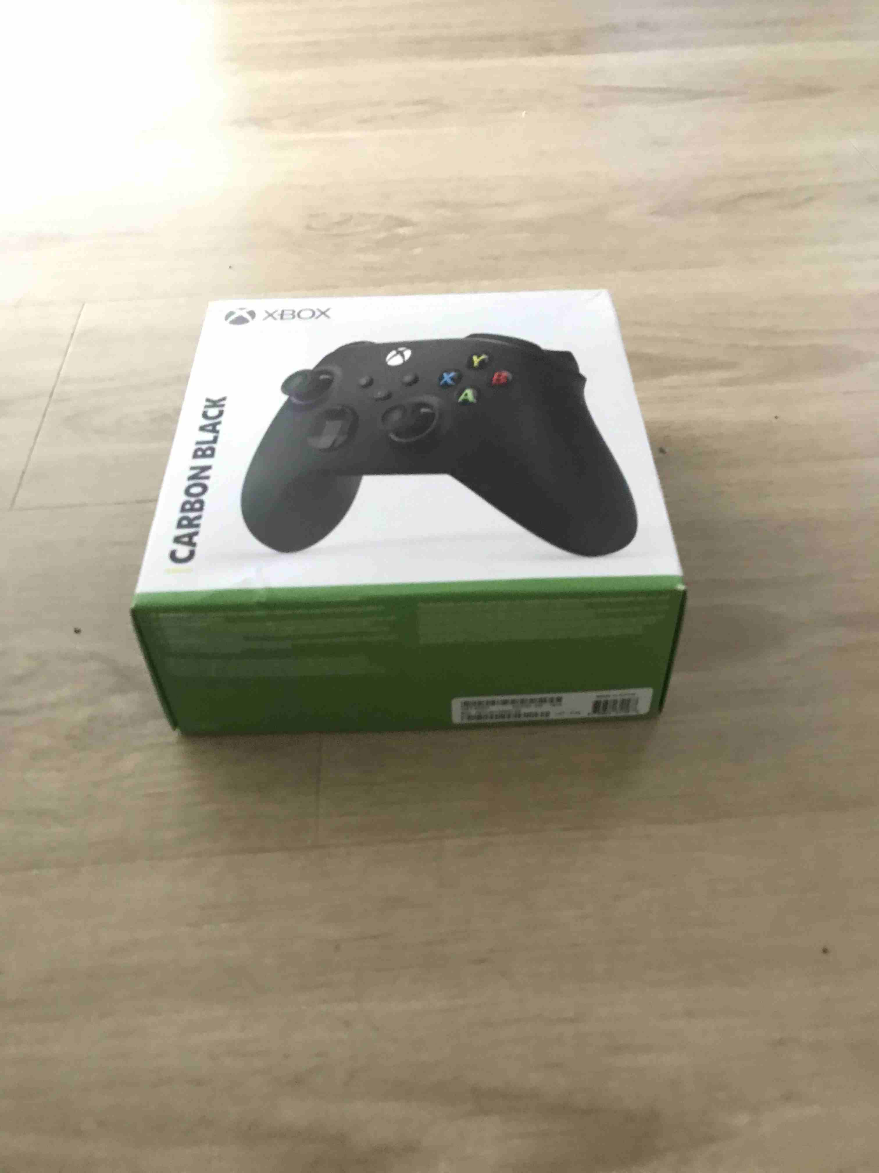 Image of xbox box before rectify
|
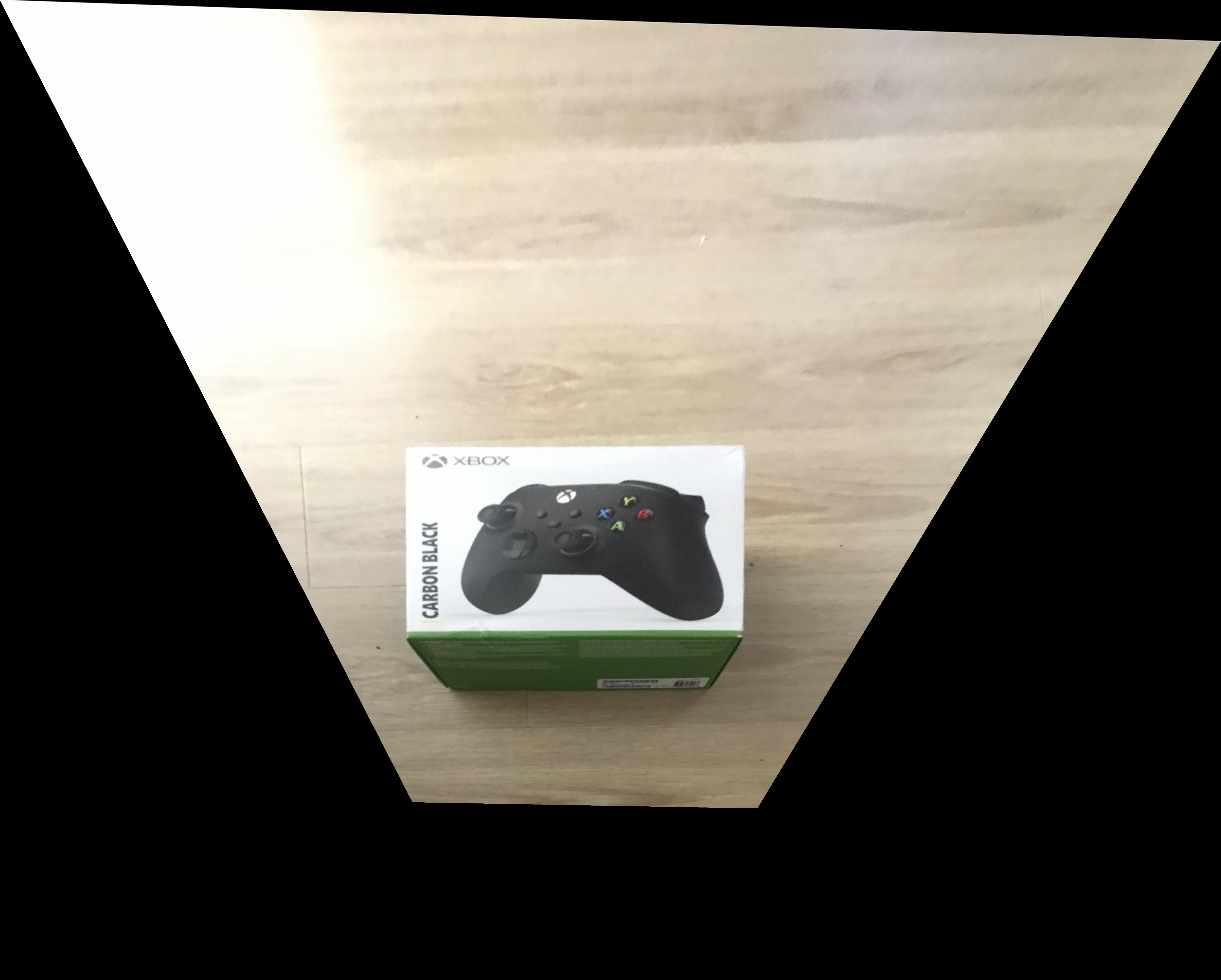 Image of xbox after rectify. It can seen that the image is straight up
|
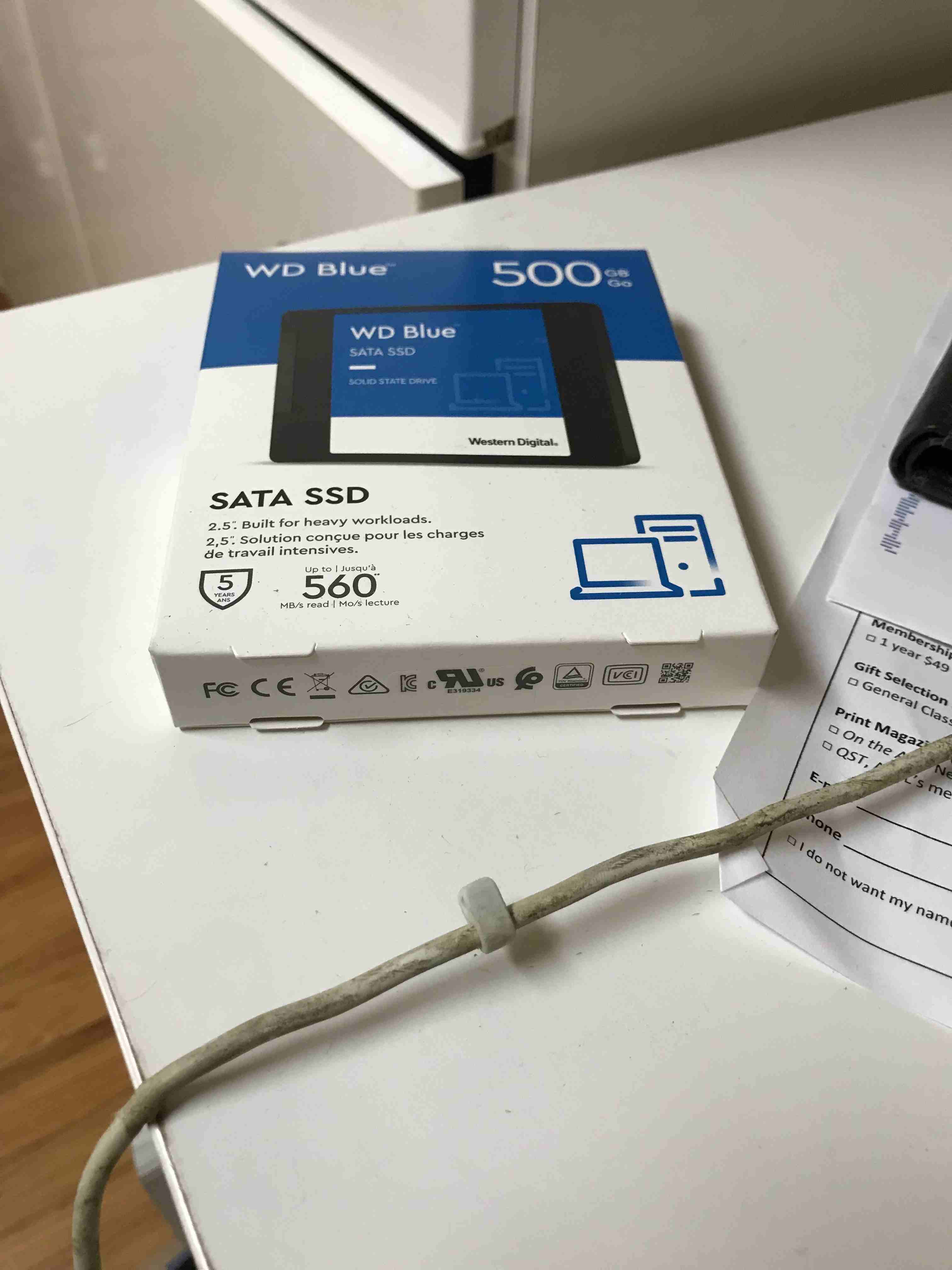 A ssd box pre rectify
|
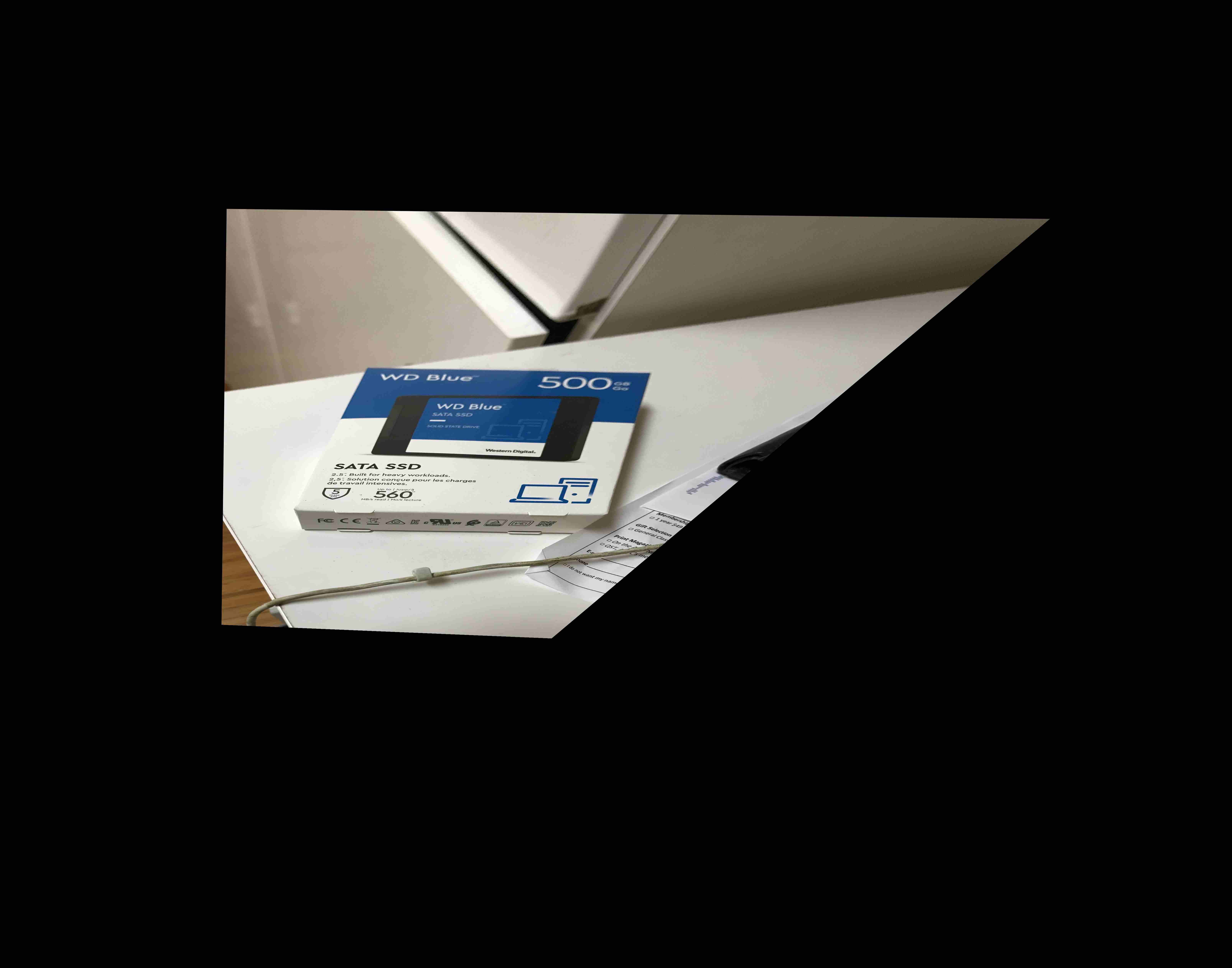 SSd box post rectify
|
.
Blending Image into a mosiac
In order to blend images into a mosiac, I just overlayed the warped image with the base image. However, this may create some sharp edges.
I created a custom process in order to produce a better blend.
First I compute mask where warp image is present, mask_a.
Then, I compute a mask_b where unwarped image is there. mask_c is the overlapping region with mask_a * mask_b.
I then compute the gaussian convolution to blur the edges for mask_a, mask_b, and mask_c. In order to reduce the overlapping region, I now subtract mask_a - mask_c and similarily with mask_b. This creates the areas that are not really overalapping with a and b but in a blurred form. Then, I compute a threshold mask of this white and black image to get the overlapped regions that is not covered by the gaussian. I blur this area with a weaker gaussian and add it to both masks. Then I multiply image a * mask_a + image * mask_b. Then, I divide by the 1/(mask_a + mask_b) to make the overlapping regions noramlized.
This process is a little confusiong, but the diagram below might help visualize what the masks are doing.
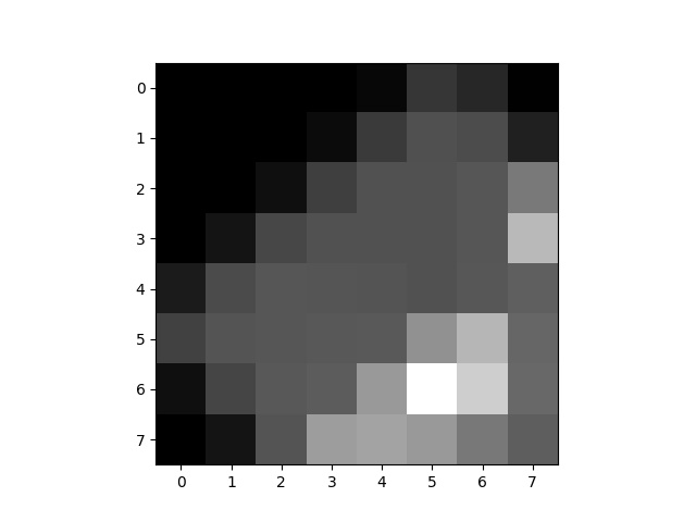
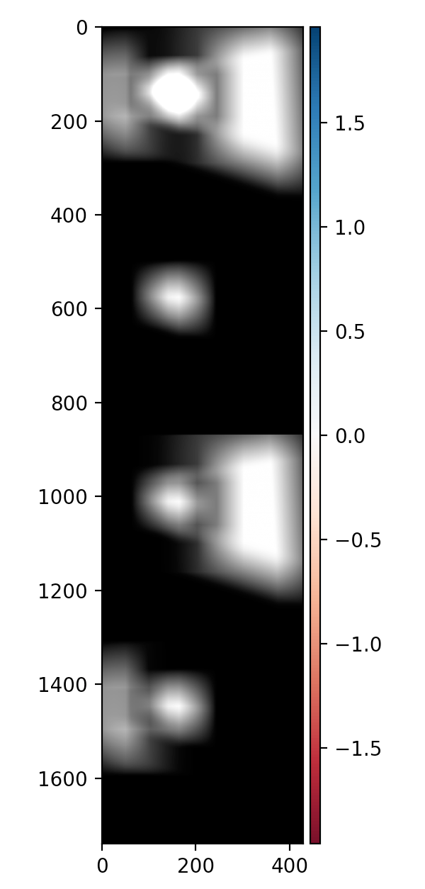 First image is mask_a + mask_b. Second image is thresholded overlapped blurred. Third is mask_a. fourth is mask_b
|
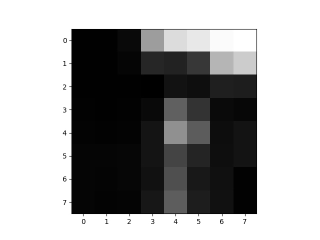
 Masks for this image
|
|
Laptop left
|
Laptop right
|
This process was convoluted but gave really good results when blurring the images.
To blend more than 2 images, I just computed the left mosiac and the then the right mosiac, then combined them together based on the offsets from the base. This can be done repeatedly.
 Complete Mosiac of my sofa
|
 Left sofa with center
|
 middle sofa with right
|
This is using the sofa images shown above.
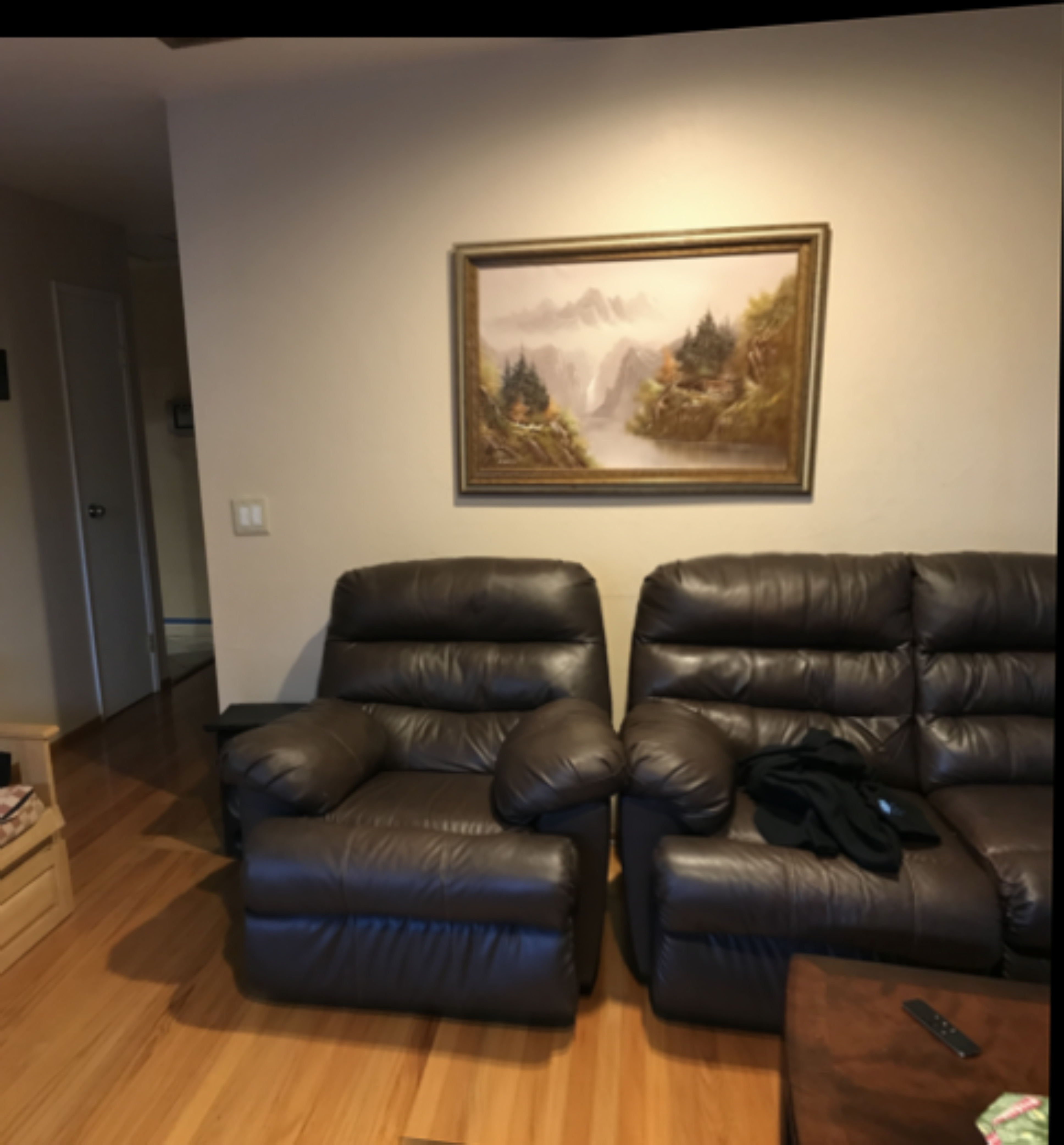
The following is with a chairs at my house.
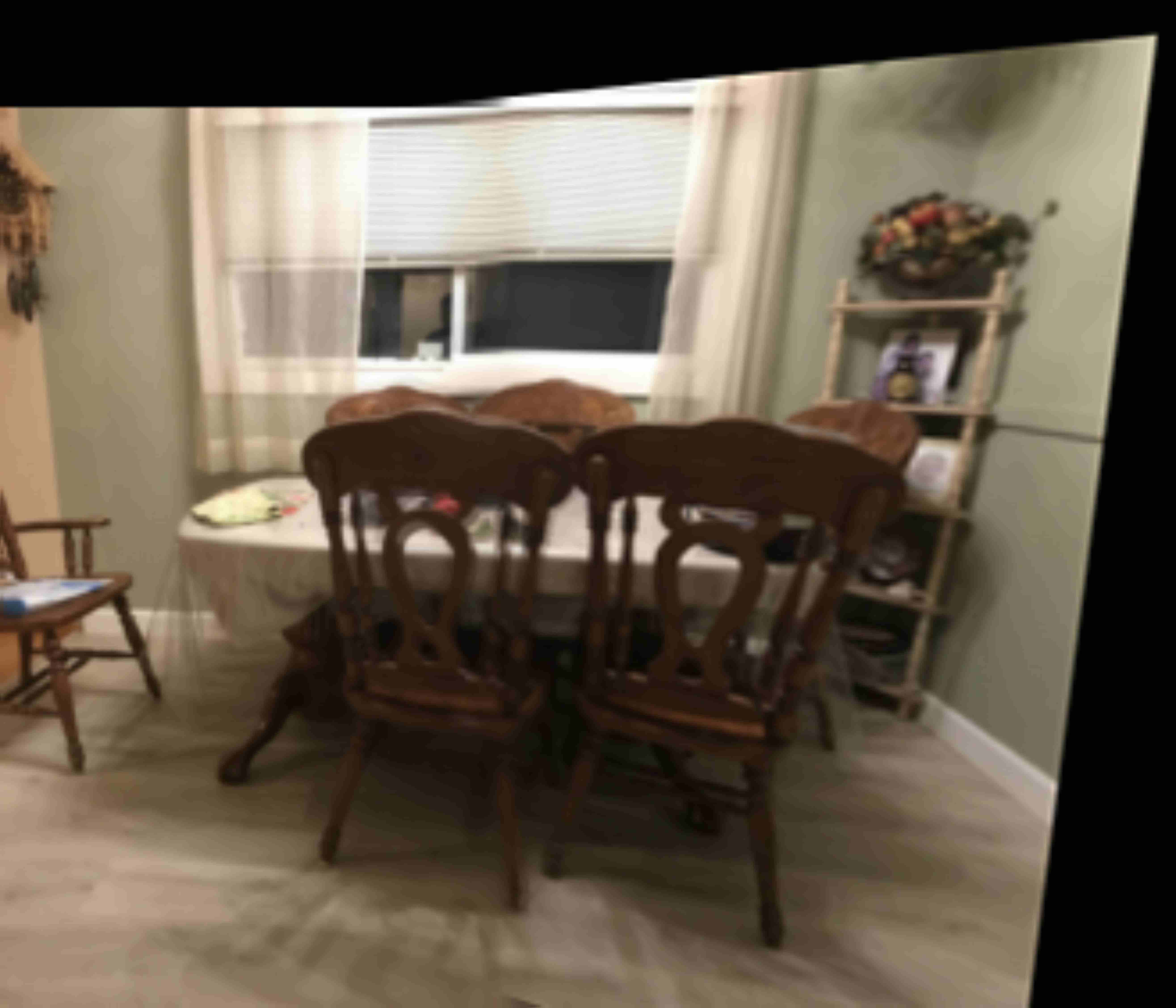 Complete Mosiac of my chairs
|
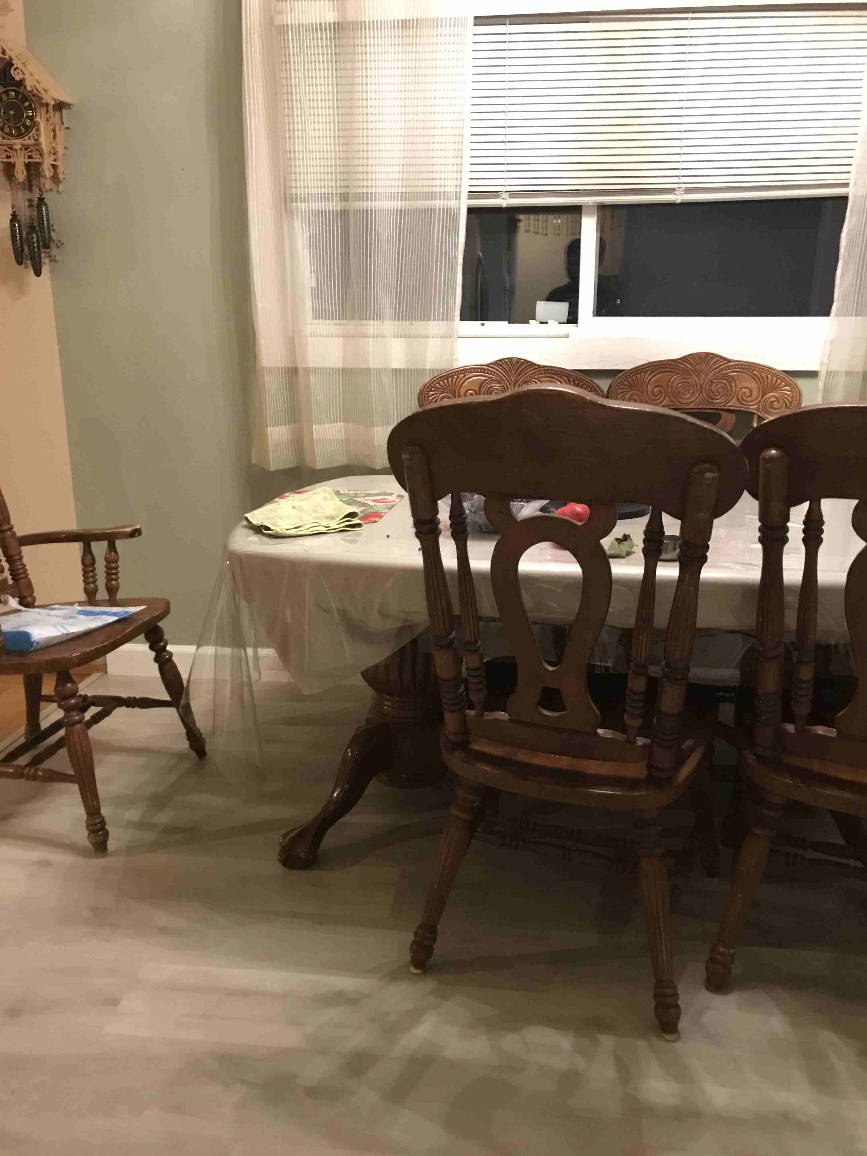 Left image chair
|
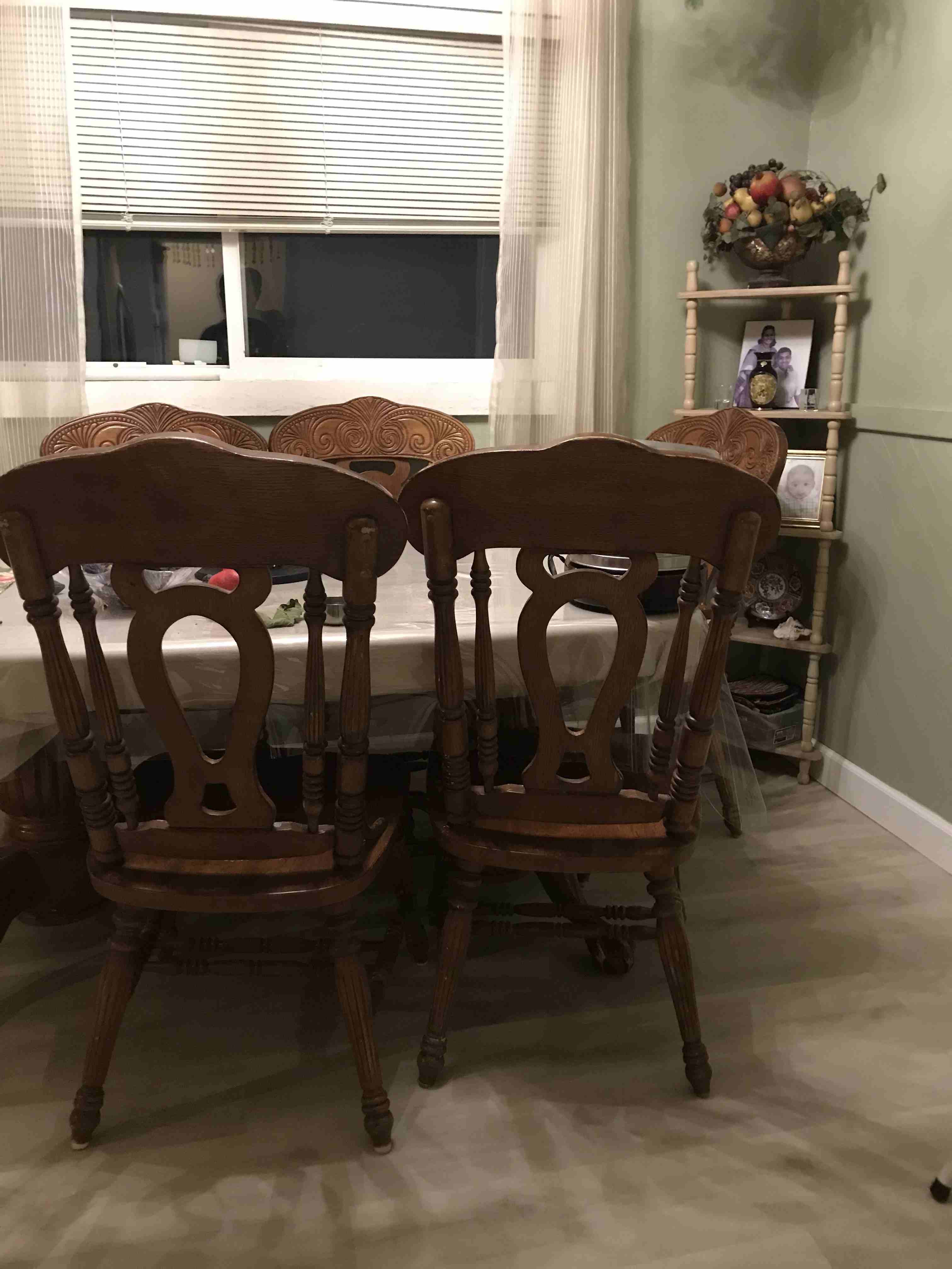 right image chair
|
Harris Feature Corner Detection + Adaptive Non-Maximal Suppression
Harris Feature Corner
Harris interested point detection works by looking at windows within the image and trying to find windows that have a change in the x and y direction.
This implies that something possibly interesting is happening at that corner, but this can be very noisy. However, this is cleaned up in later.
Adaptive Non-Maximal Suppression
The goal of Adaptive Non-Maximal Suppression(ANMS) is to reduce the number of points considered. given the strengths and coords from harris, we loop through every coordinate.
For each coordinate, we filter out coordinates that have coordinate's harris value <= .9 * other_coordinate's value to create a list of valid coordinates. Then we compute the smallest radius to the points that are valid.
This is the same as performing the following objective function.
 ANMS formula
|
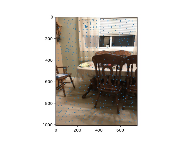
The following is the completed anms and harris coordinates.
|
Complete Mosiac of my chairs
|
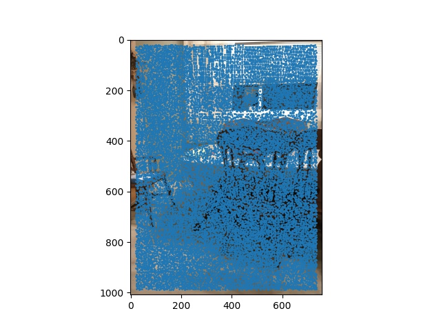 Left chair with harris points
|
 left chair anms
|
Feature descriptor Extraction + Feature Matching + Bells and Whistle for Feature Extraction
Once we compute the anms, we have a filtered list of coordinates.
We want to try to get the different patches of the images around the coordinate normalized.
We first take the points (-20, 20) around the coordinate and then normalize it.
For some images, they need to be rotated when stiched together. This can be done by rotating the patches before comparing it.
We first compute the gradient in y and x with sobel filters. We then compute arctan(y/x), crop, and then rotate the patch.
This rotational change especially helped a lot when creating mosiacs with images slightly turned.
To match features, we take every point of image 1 coordinate, and then take every point of image 2 coordinates. We then compute the distance between the descriptors. We then sort the distances and compute the distance[0]/distance[1], which represents the 1-KNN/2-KNN.
This has be shown by the paper in lecture to be a good indicator of true positive points.
We then validate it's a pair if the ratio is less than a hyper paramater threshold. For most images, a threshold of .2 worked.
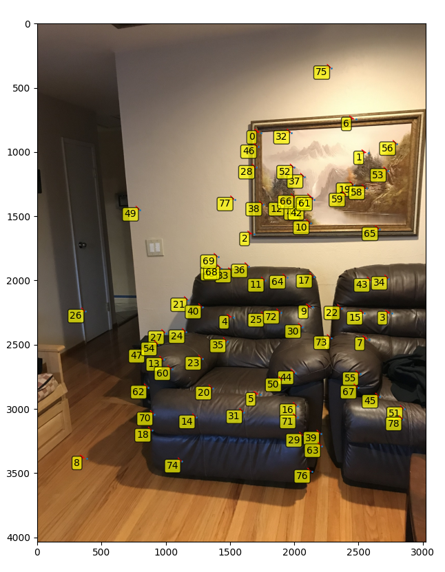 Left chair matched without rotation
|
 Center sofa matched without rotation
|
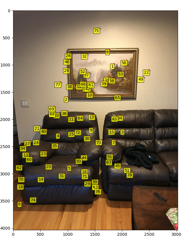
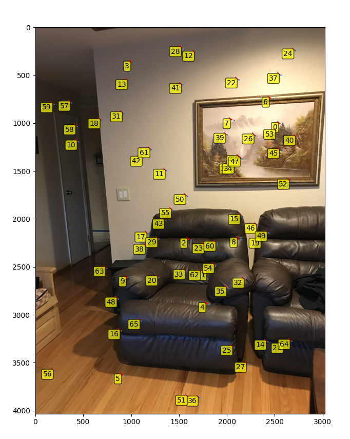 Left chair matched with rotation
|
 Center sofa matched with rotation
|
 Feature descriptor plotted for one part of an image
|
 Feature descriptor plotted post rotation
|
From the above, you can see the the points are matched relatively accurately. The false points can be fixed via ransac. \
It can also be seen from these images that the rotation change picks up different points that the non rotational misses.
Ransac
After computing the matching pairs, the ransac algorthim is used to find the best set of coordinates.
This involves first choosing 4 points in img1 and corresponding in img2, computing a homography, and then finding the number of points that in img1 that are close as img2 in transformed space. The distance threshold used is .5 for most cases. We collect the number of points that match and repeatedly apply this random selection for a certain number of iterations(I use 10,000).
The largest set of these points(inliners) is used to compute the final homography.
With this homography, we pass it into the previous parts blending code. In order to blend more than 2, we repeatedly compute blend of consecutive images and then blend the resulting of those images(n^2 approach).
These operations can all occur in parallel.
The following are results of ransac and comparing them to the manual approach.
 Auto left sofa with center sofa blended
|
 Auto center sofa with right sofa blended
|
 Auto mosiac with the sofa image used before
|
manual mosiac with the sofa image used before
|
 Auto chair matched. Note that the ransac sometimes has issues with similar brown patches.
|
Manual chair matched
|
Note the laptop from earlier parts wasn't included since it involved heavy rotation and a lot of similar colors between the images, making the current approach detect a lot of false positives.
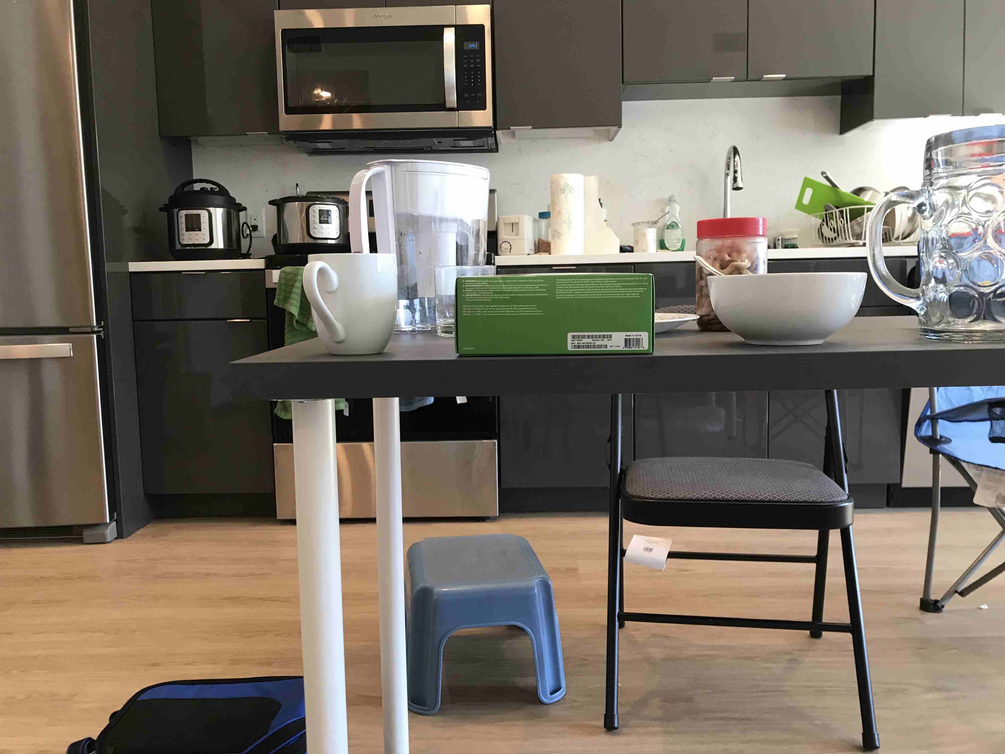
Instead we can look at this image of a kitchen. The exact image are slightly rotated and shifted.
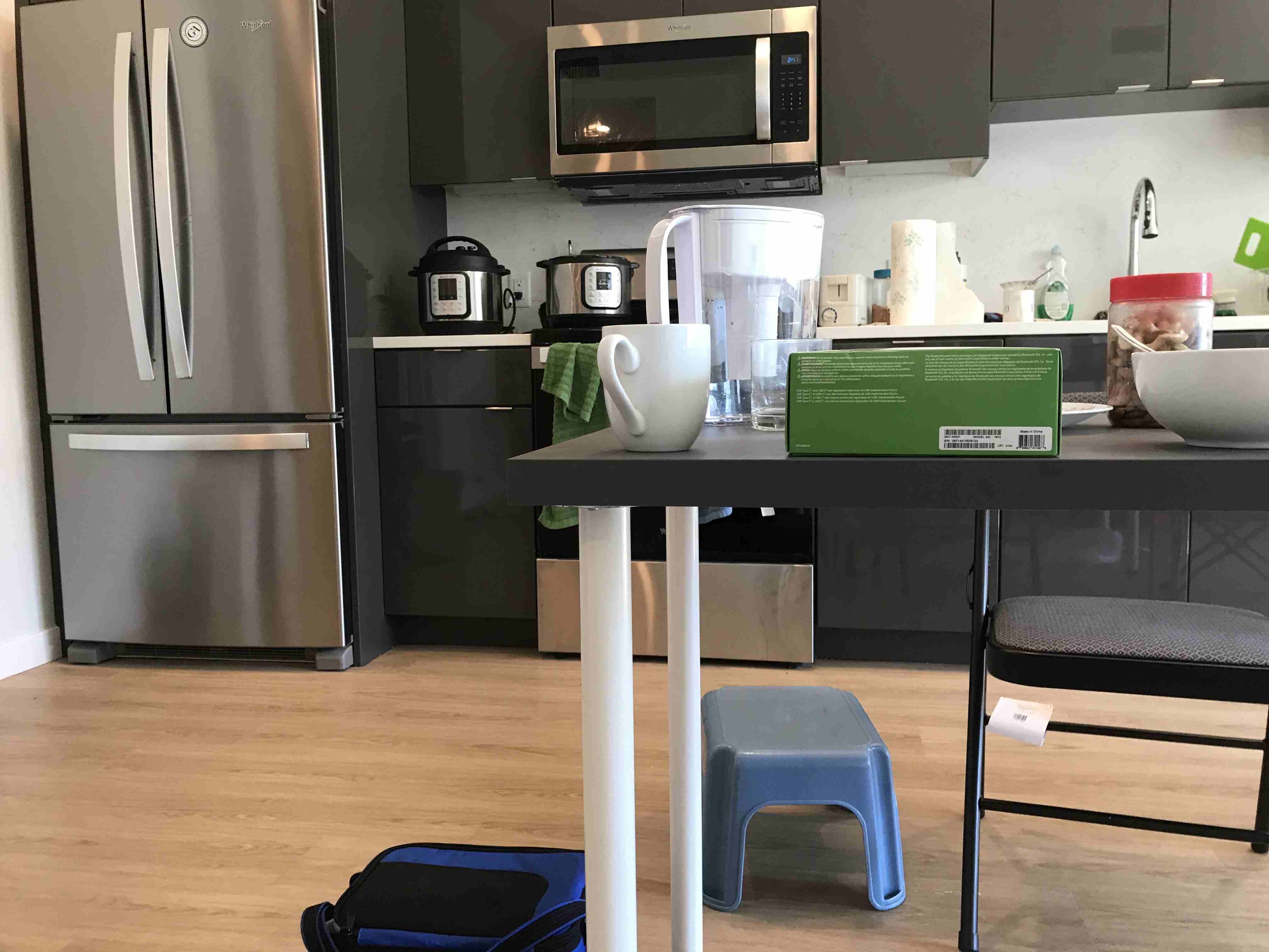 Kitchen Left
|
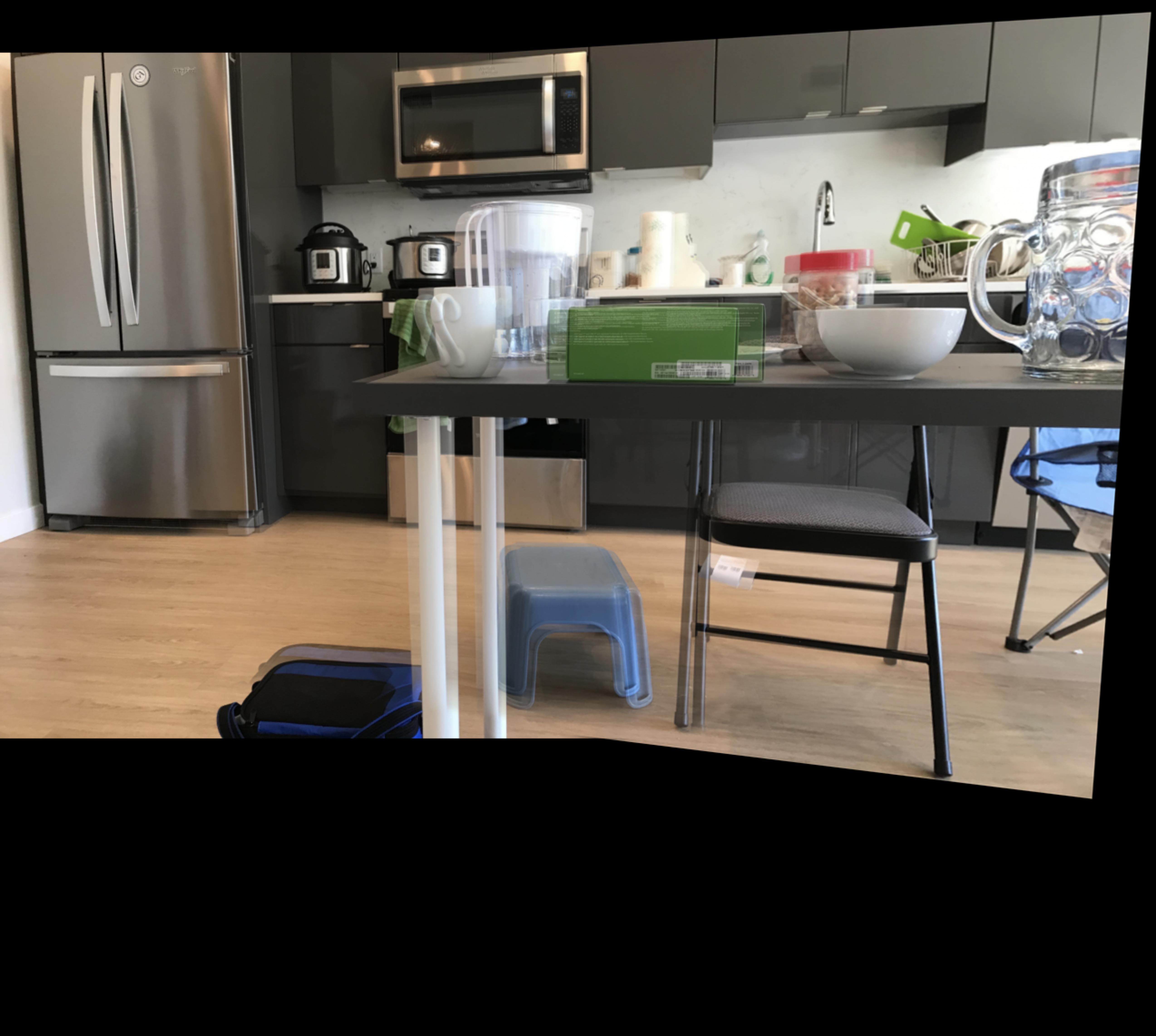
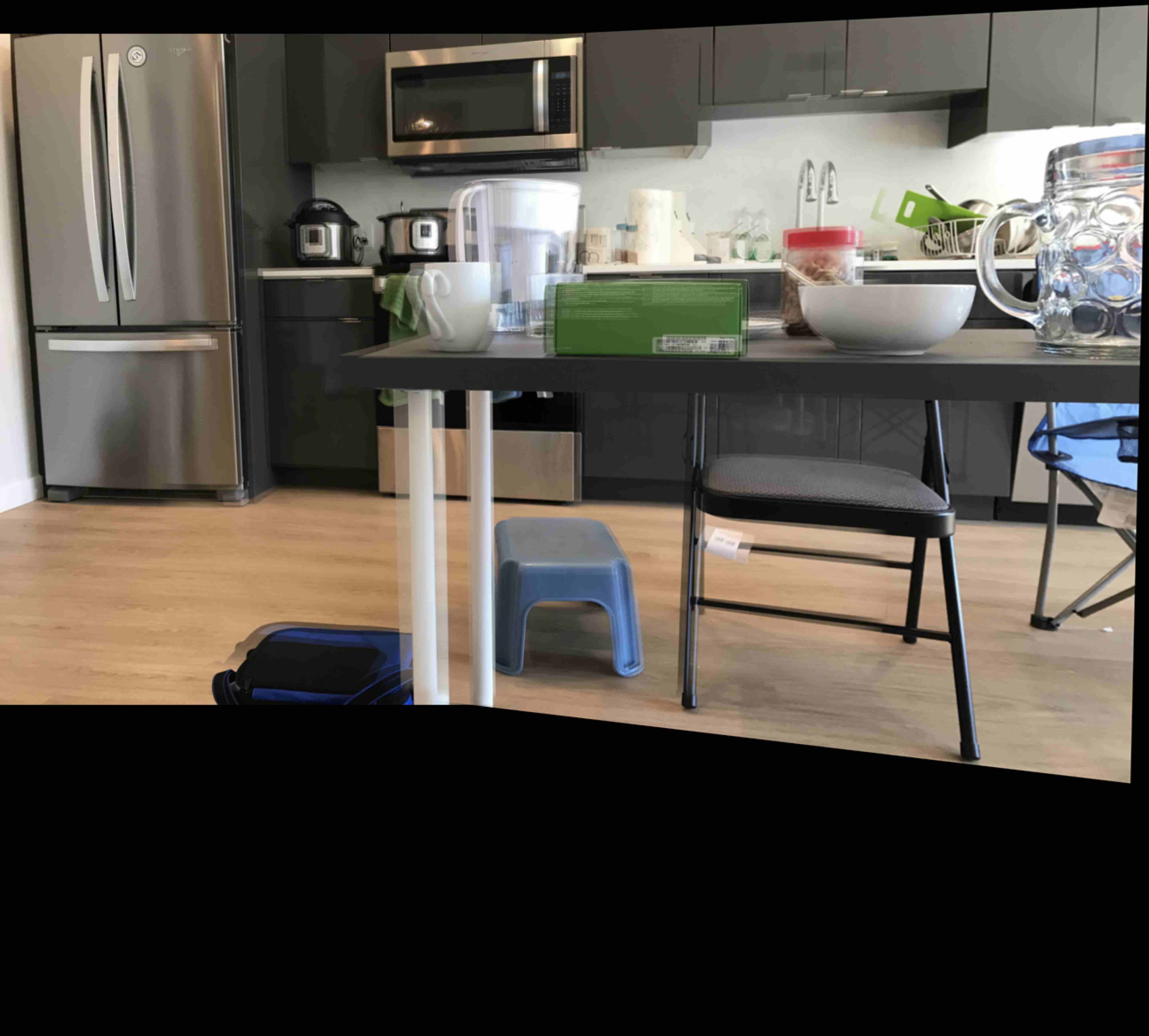
 Kitchen Right
|
 Auto blended kitchen
|
 Manual Blended kitchen
|
Overall, the auto version in the sofa was much better due to distinct set of colors. The auto seems to be fail if there are patches of similar color.
Conclusion: What have you learned?
I learned a lot about auto alignment and patch detection. The idea behind autoransac was really interesting, repeatedly trying transformations till a solution is viable. This seems like it can be applied to other algorthims as well.
The auto blending looked reasonable and saved a lot of time manually selecting points.