Photo Mosaics
COMPSCI 194-26: Computational Photography & Computer Vision
Professors Alyosha Efros & Angjoo Kanazawa
October 14, 2021
Ethan Buttimer
PART A
Overview
In this project, we learned how to compute homographies and use them to warp images. We could then stitch these images together (with some clever blending techniques) to create an image mosaic! These mosaics can appear to be taken from a single viewing angle, when in fact they are made of a collection of images taken from different angles.
My favorite part was learning how to compute the homography from a set of correspondence points. It was cool to use least squares on a greater number of points to compute a better set of transformation parameters!
Shooting the Pictures
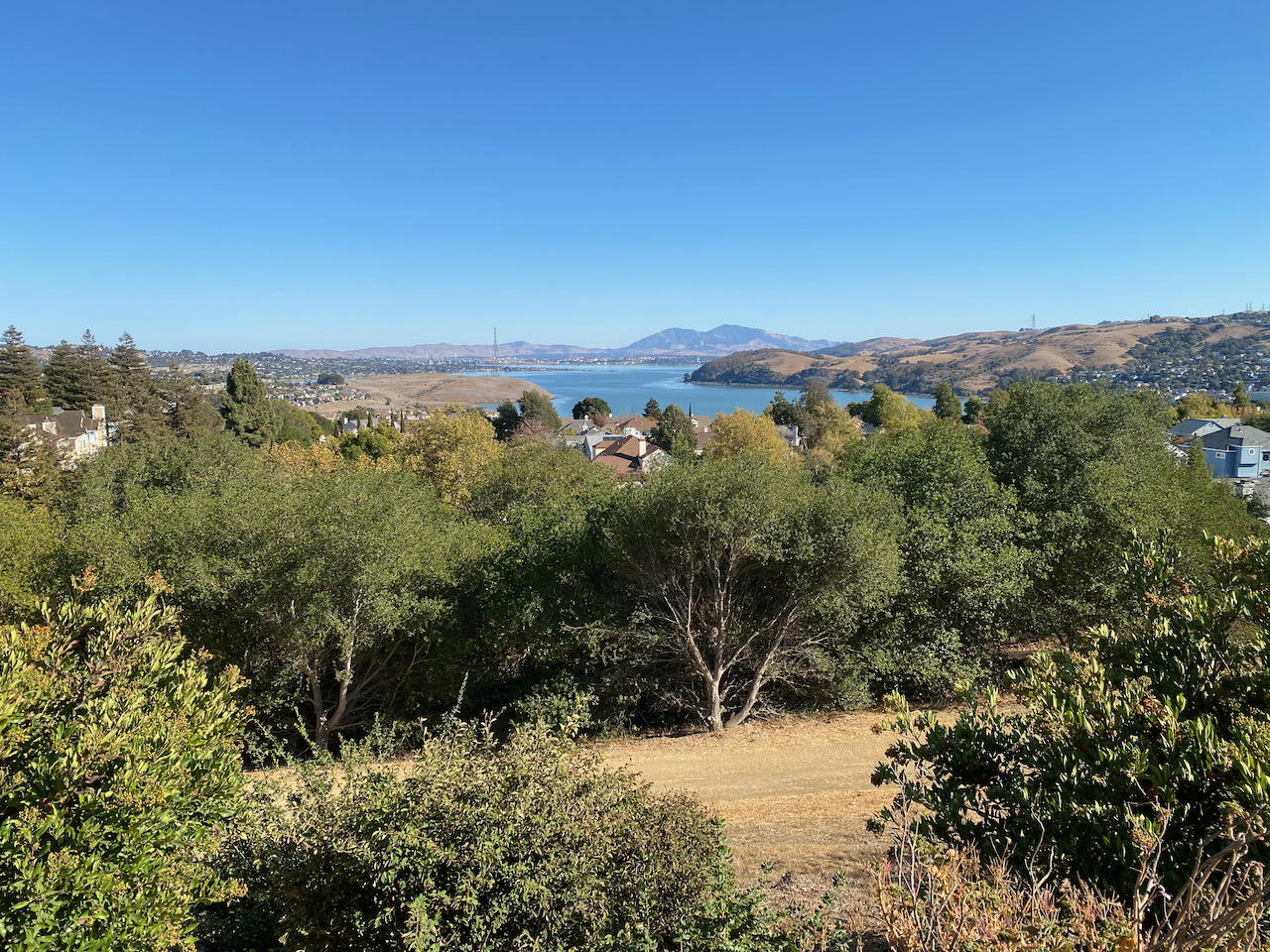
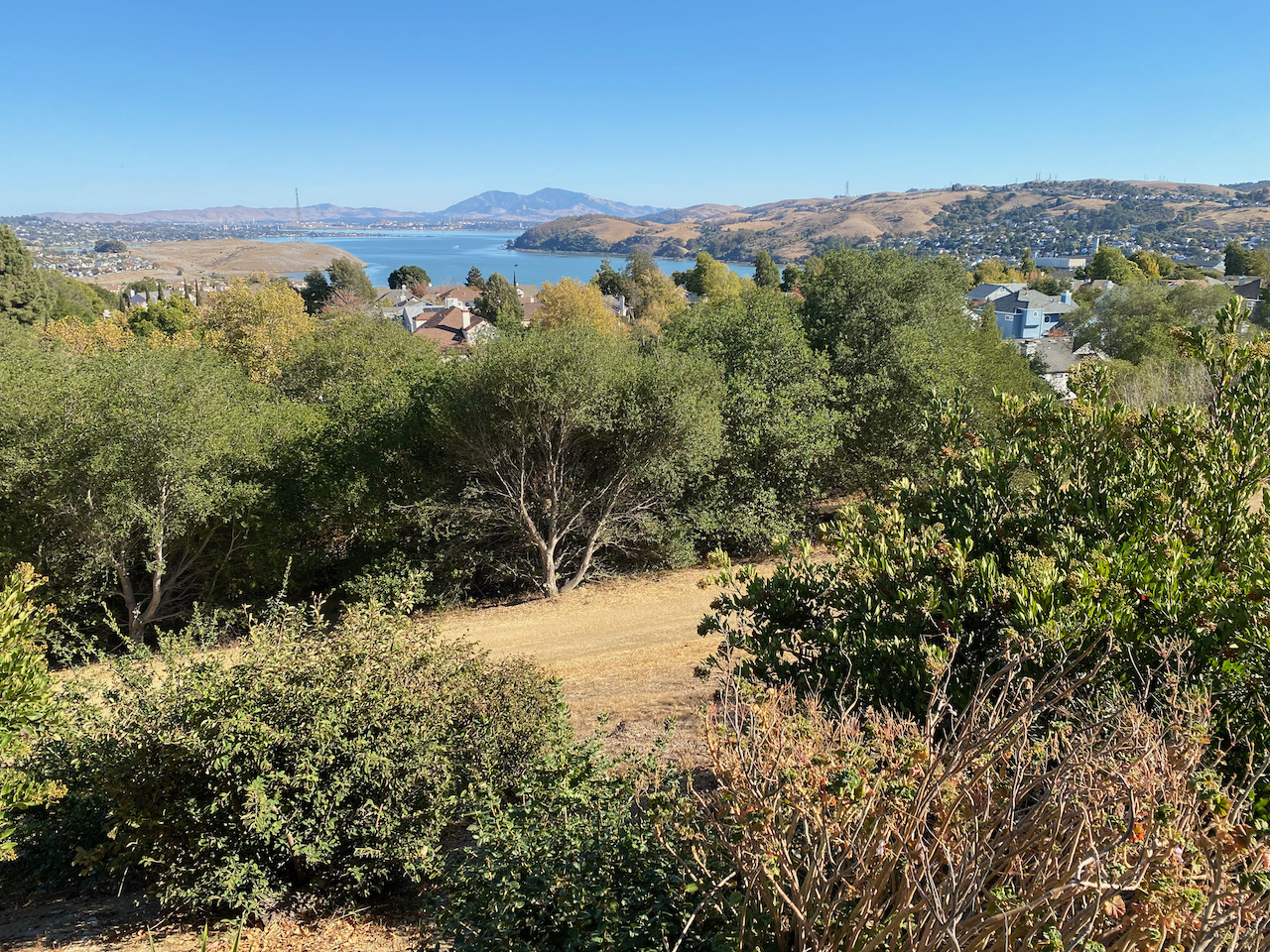
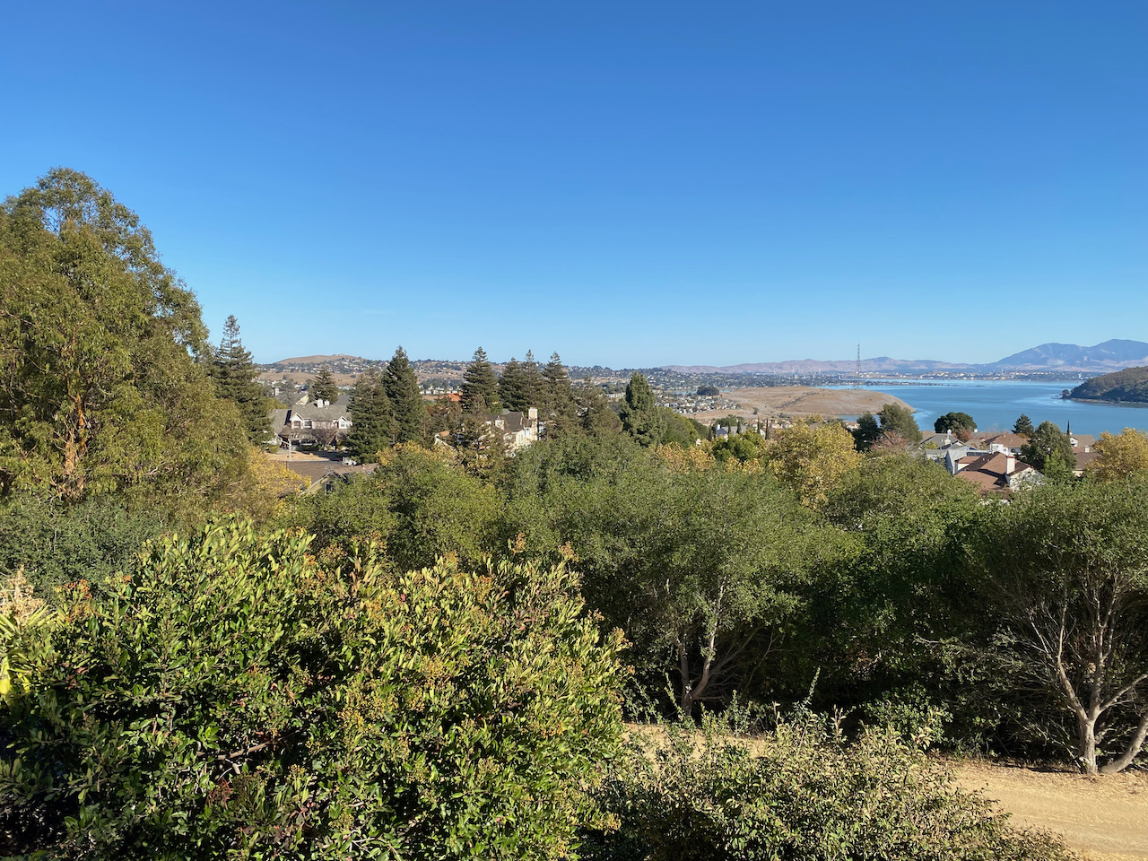
I shot all of the images used in this project on my iPhone 11 camera at the default focal length and with locked exposure. The images used for a mosaic were all taken from the same camera location with ~50% overlap at different rotations.
Recovering Homographies
To define a homography between two images, at least four points of correspondence must be selected. Then, using the method detailed here, I could compute the parameters of the 3x3 homographic transformation matrix. This matrix allowed me to warp one image such that it appears to have been taken from the camera angle of different image. I also implemented least squares in order to compute the optimal transformation given more than four points (which results in an over-constrained system). I often saved correspondence points to JSON so they could be reused.
Warping Images
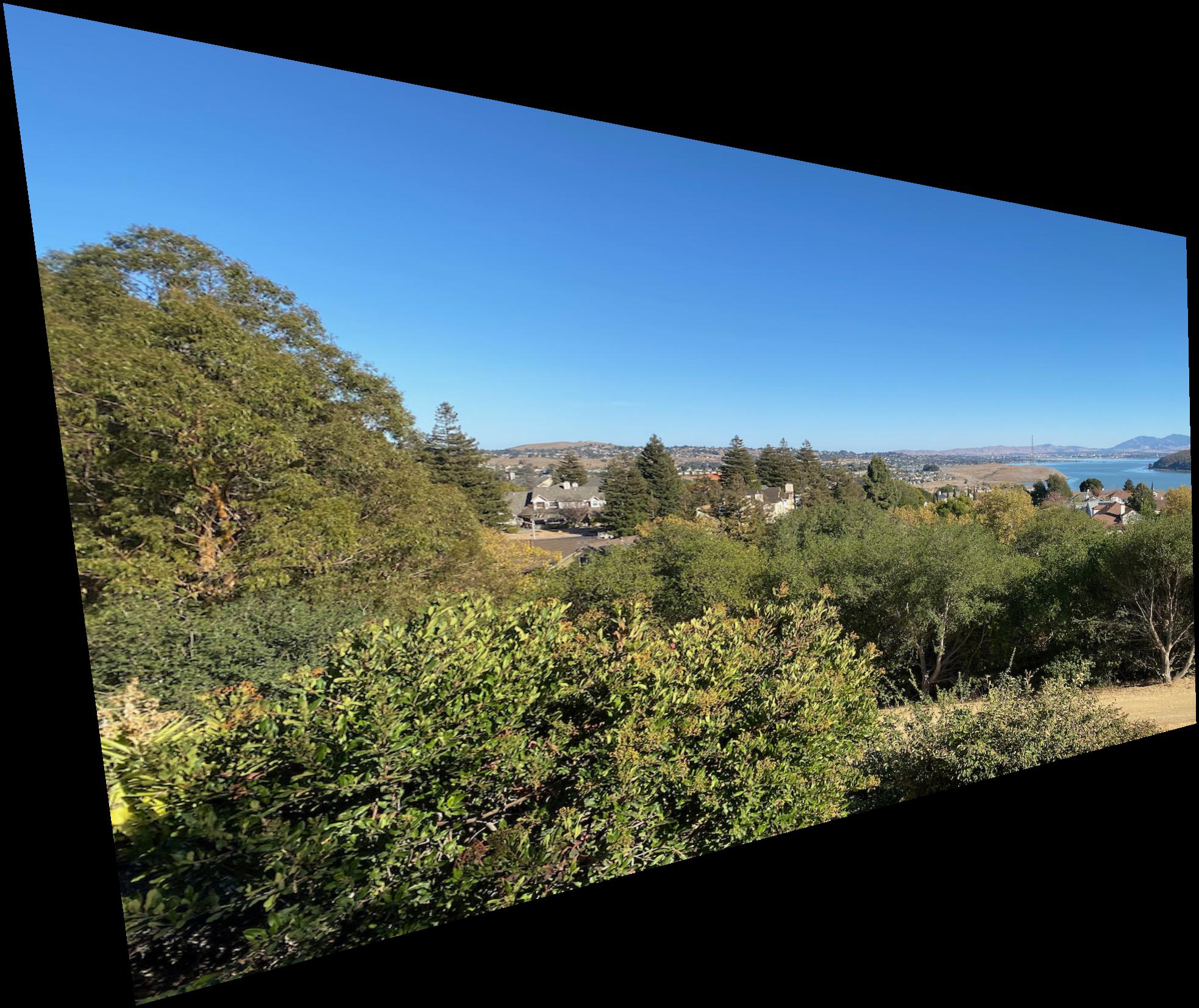
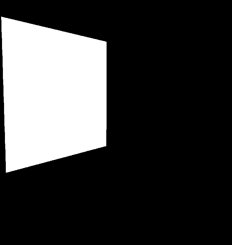
I began the warping process by computing the corners of the warped image (by multiplying my the homograpy matrix and rescaling). I then created a binary alpha mask using these corner coordinates. I then gathered the coordinates of the pixels inside the mask and applied the inverse homography to them. The transformed coordinates were then used to sample from the unwarped image using bilinear interpolation, and the final warp image was assigned these colors.
Image Rectification
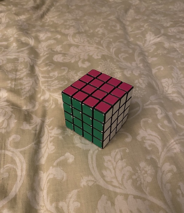
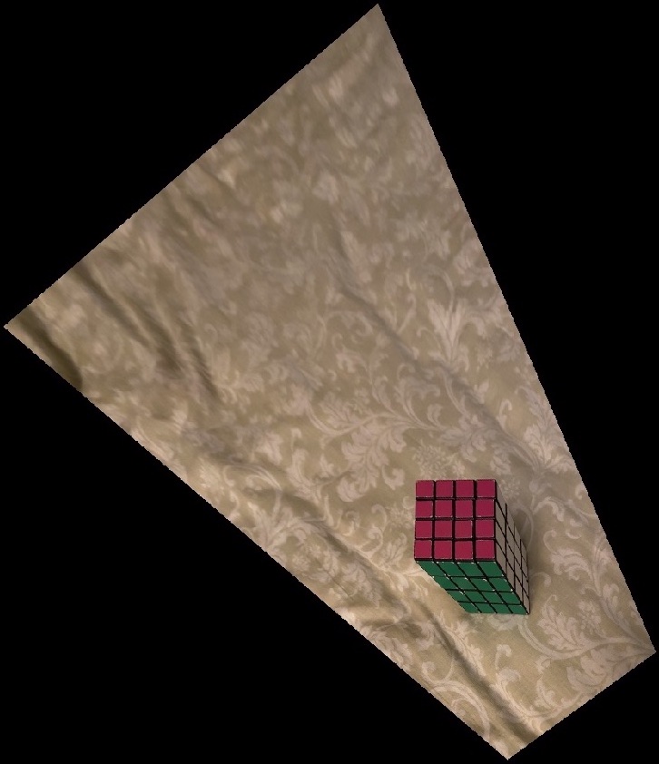
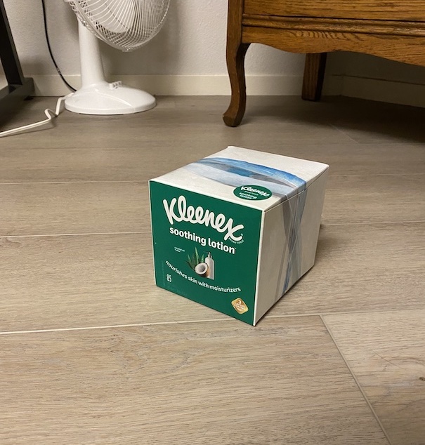
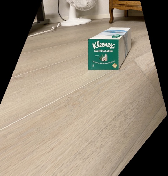
Using a correspondence between a square surface in an image (viewed as a non-square quadrilateral) and a manually defined square, I could compute a homography to warp a source image such that the chosen surface takes the shape of a square. This "image rectification" technique is shown below, performed on the pink surface of the Rubik's cube and the bottom of a tissue box (note: the images below have been cropped).
Mosaic Creation
I formed my mosaics iteratively, adding a single warped image to the full mosaic each time so that new correspondence points could be defined if necessary.
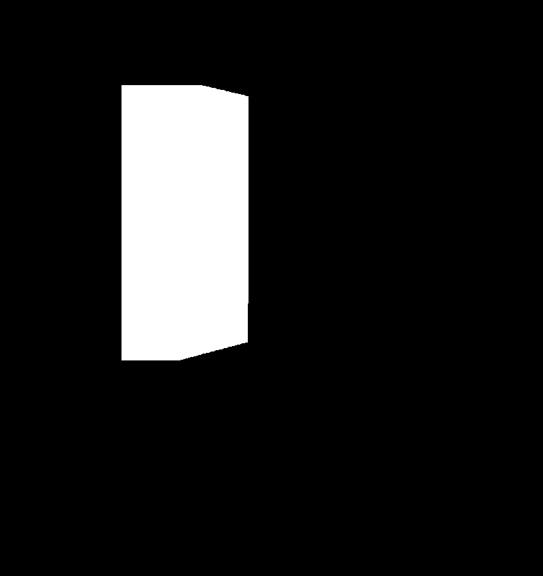
On a single iteration, the mosaic (or starting image) remained fixed, while the new image was warped. Then, I computed constraints on the bounds of the mosaic to be formed using the offsets returned by the warping operation. I also generated masks for the current mosaic and the new warped image.
| Illustration of Blending Operations |
| New mask |
Existing mask |
Overlap |
 |
 |
 |
| New mask, minus blurred overlap |
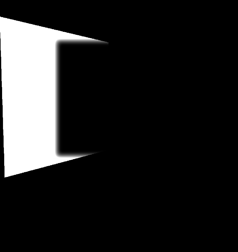
Existing mask, blurring along edge of overlap |
Existing mask, fully blurred |
 |
 |
 |
| Color contribution of new image |
Color contribution of existing mosaic |
Added result |
 |
 |
 |
To blend the images together, I first found the overlap of the two masks. Next, I found the masks of the two image without the overlapped area (by subtraction). I then created two special masks: one for the current mosaic, with a blurred boundary only along the boundary of the overlap zone, the other for the new image with a blur only along this same boundary. Creating these two masks involved clipping and scaling the range of a Gaussian blur, and a few mask subtraction operations. Finally, I multiplied each of these masks by the corresponding (transformed) image, and added them together to get the new blended mosaic for that step! I chose this method of blending only along the edges so that as much of the mosaic as possible could consist of pixels from just one image, rather than a blend of two or more. Below, I've shown how my method compares to simple pixel replacement on one mosaic.
PART B
Overview
For the second part, I implepented automatic correspondence generation (rather than hand-picking points of correspondence). This involved detecting and extracting features, then matching and filtering these corners with ANMS and RANSAC.
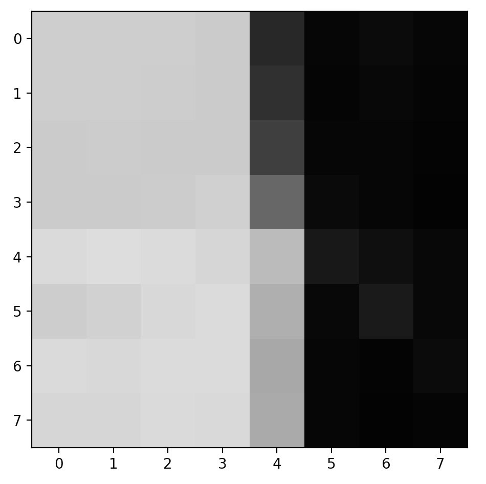
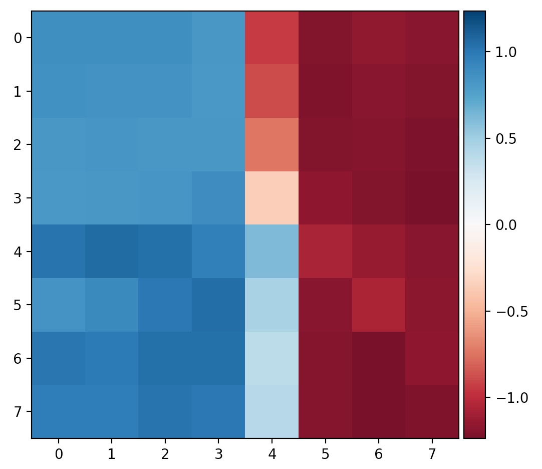
The coolest thing I learned from part B was how to find translational and bias/gain invariant features. The correct matches over these 8x8 patches had a surprisingly small SSD value and act as a great way to distinguish features.
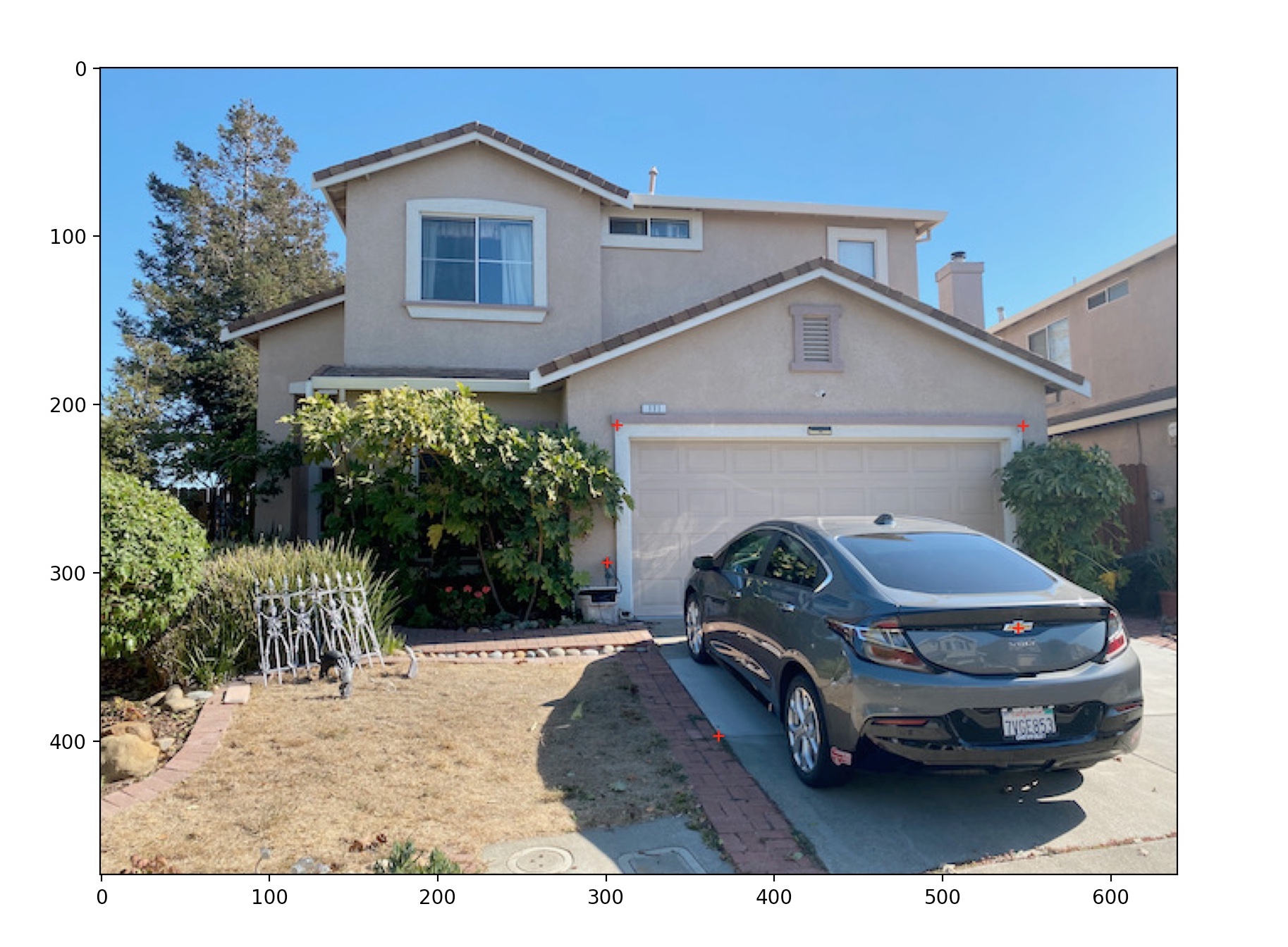
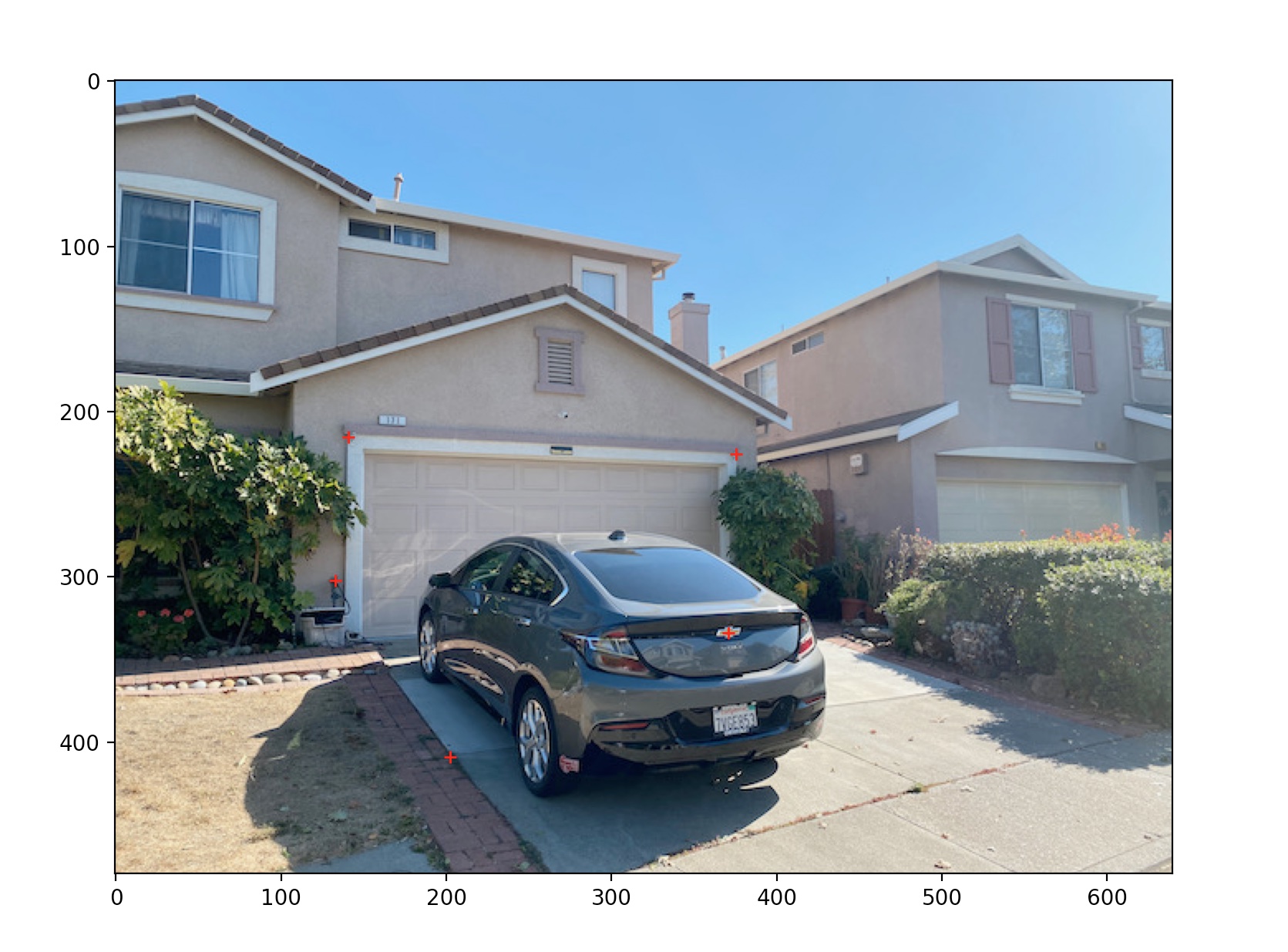
Detecting and Selecting Harris Corners
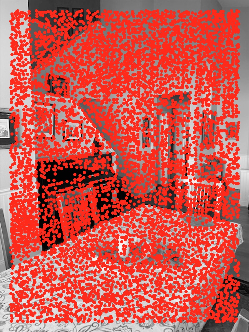
I used a pre-defined method to compute the initial Harris corners. Above, I've shown these (completely unfiltered) Harris corners on a single image. Note that I've purposefully excluded points along the edges of the image.
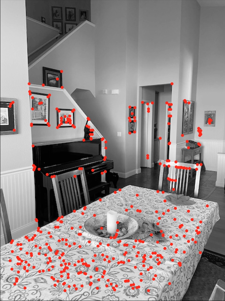
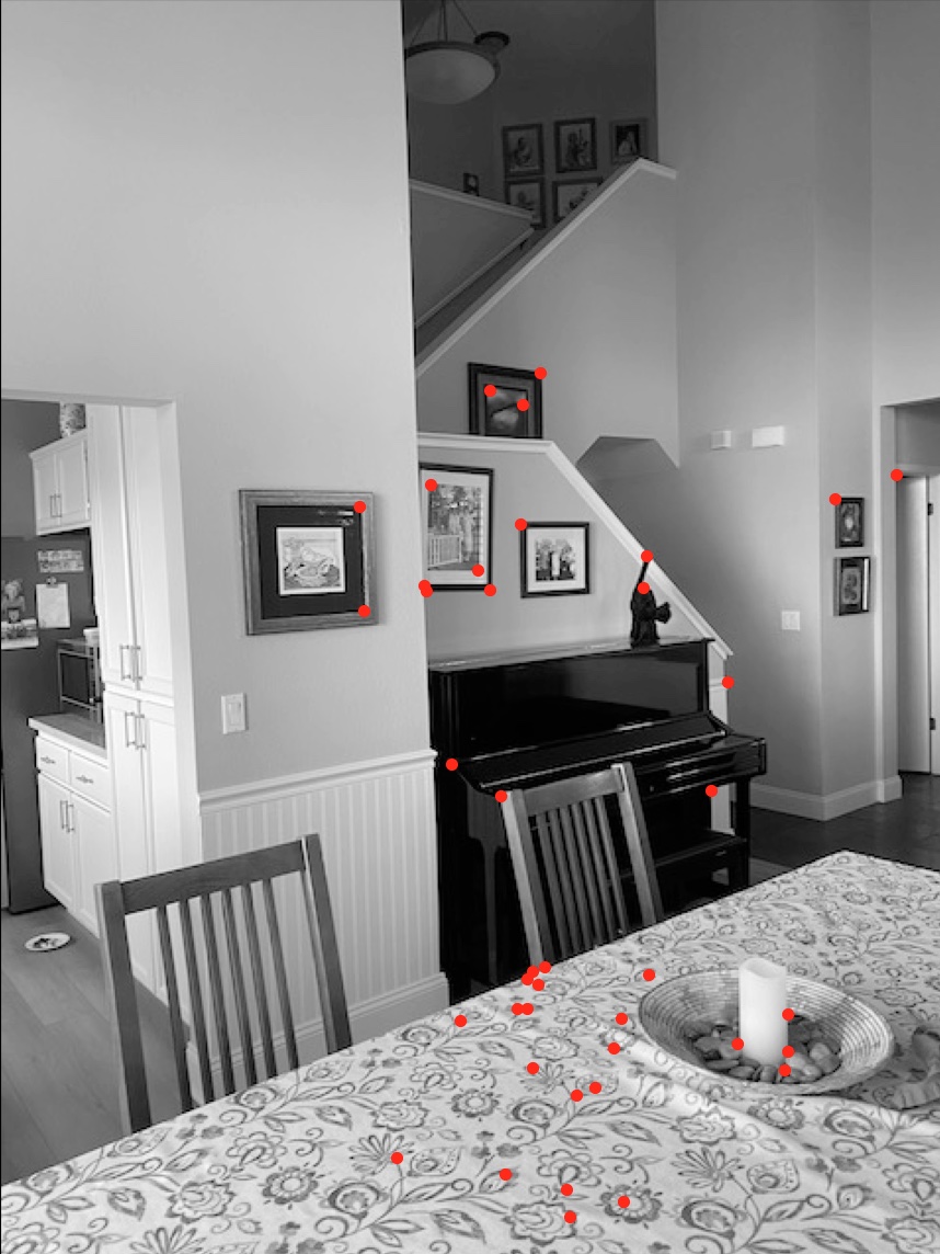
I then used the Adaptive Non-Maximal Suppression (ANMS) algorithm to pick the best 500 Harris corners generated on the image. This gave me a set of points with high Harris corner-variance values and a balanced spread across the image. This filtered collection is shown above.
Note: my ANMS algorithm was causing errors so I switched to selecting the 500 points with the greatest Harris corner values, regardless of relative position.
Matching Features
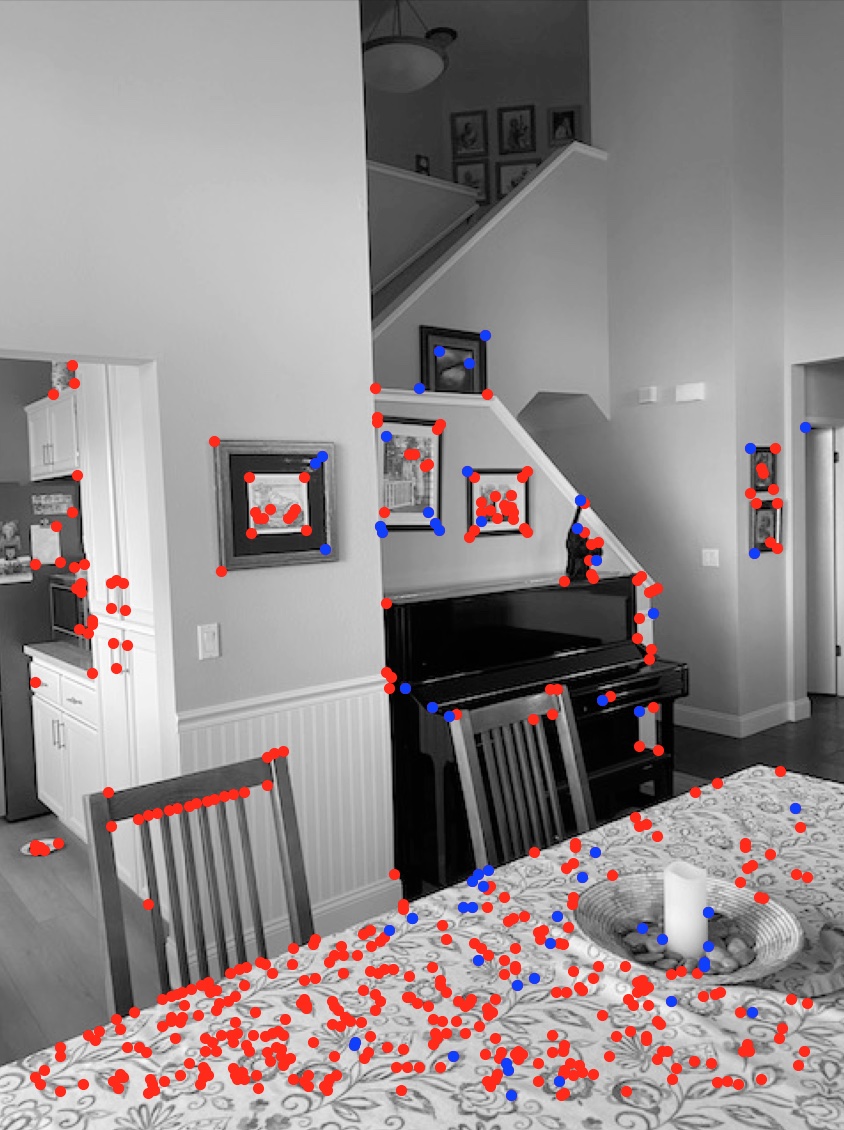
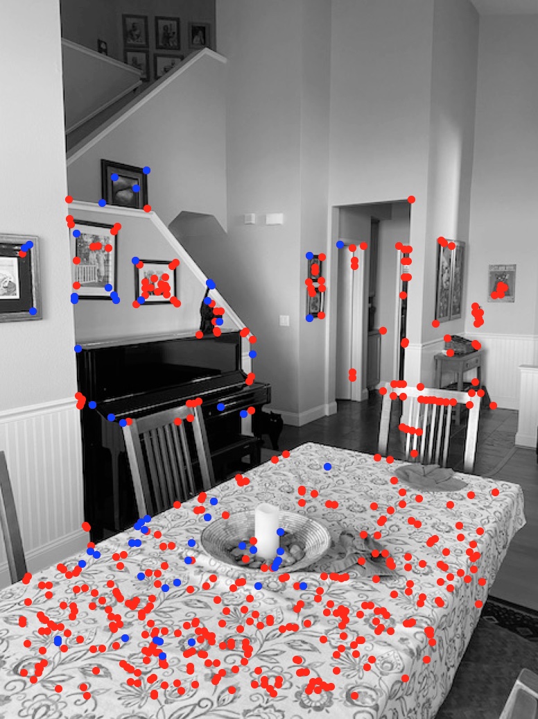
To pair up the Harris corners between the two images, I computed the SSD between each of the 8x8 features and sorted them using these SSD values. I then found the two nearest matches for each feature and computed 1-NN / 2-NN, where 1-NN is the SSD of the first nearest, and 2-NN is the SSD of the second nearest. I rejecting pairs where 1-NN / 2-NN > 0.4 in my implementation of Lowe's Trick.
Computing Homographies with RANSAC
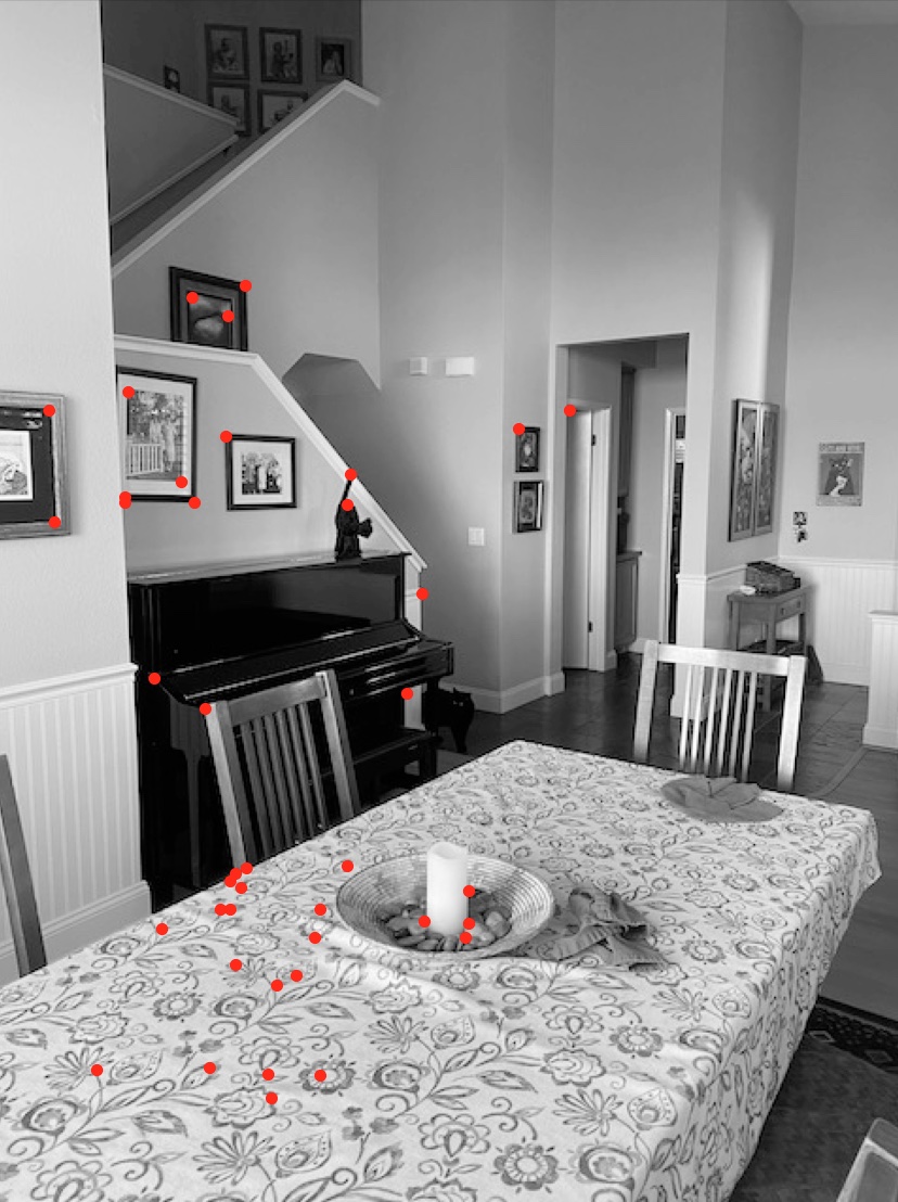
The final step to find matching correspondences and the homography between the images was RANSAC. For a fixed number of iterations (I usually used 100), four pairs of correspondences are selected and the homographic transformation between them is computed. Then, this homography is applied to all of the corner coordinates for one image, and these are compared to the unwarped coordinates for the other image. If the distance is less than epsilon (I usually used 1 pixel) then it is considered an inlier and added to a list for that iteration. The maximum-length inlier list is used to get the final correspondence points and thier homography (computed with lwast-squares over all inliers).
RESULTS
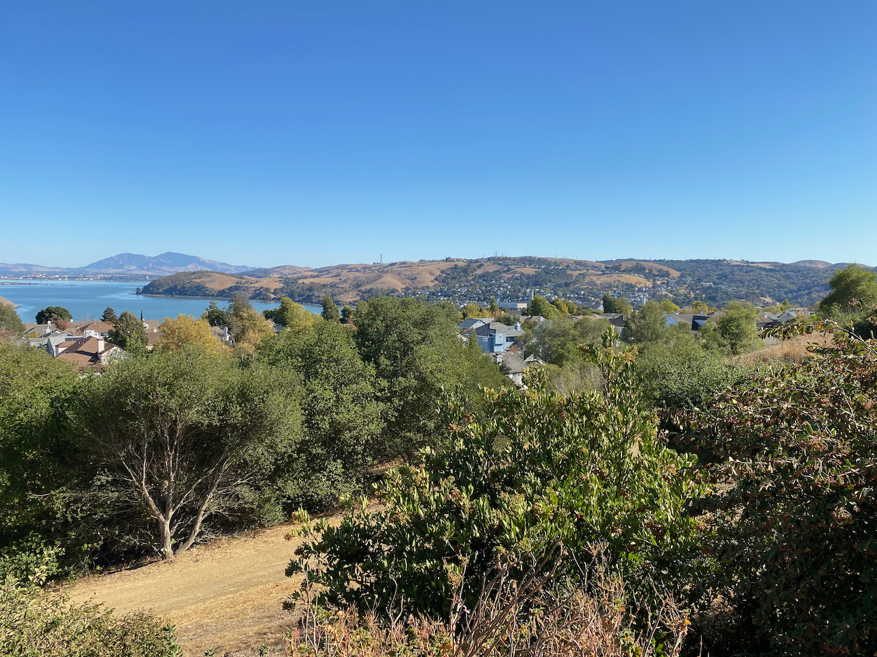
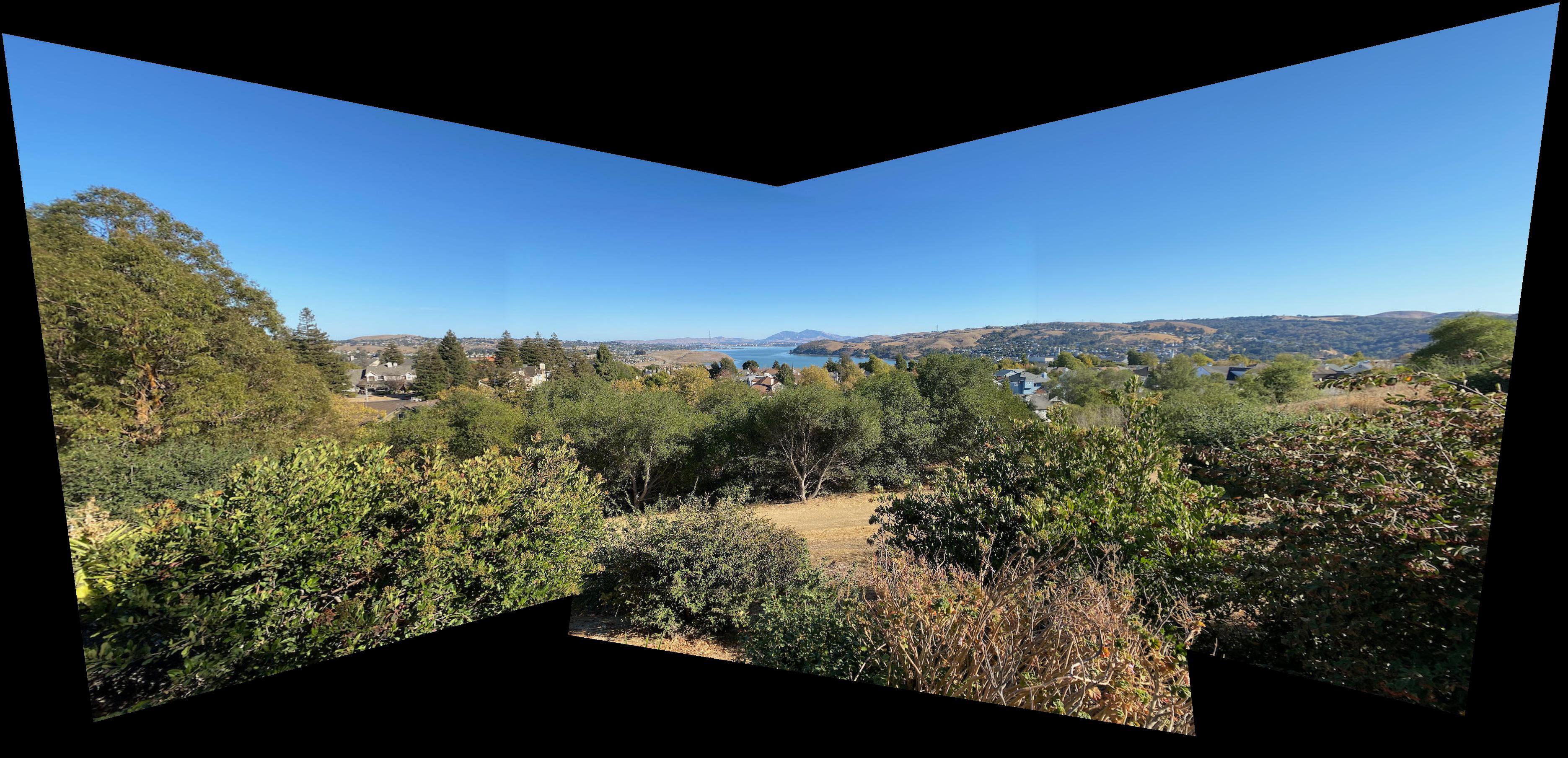
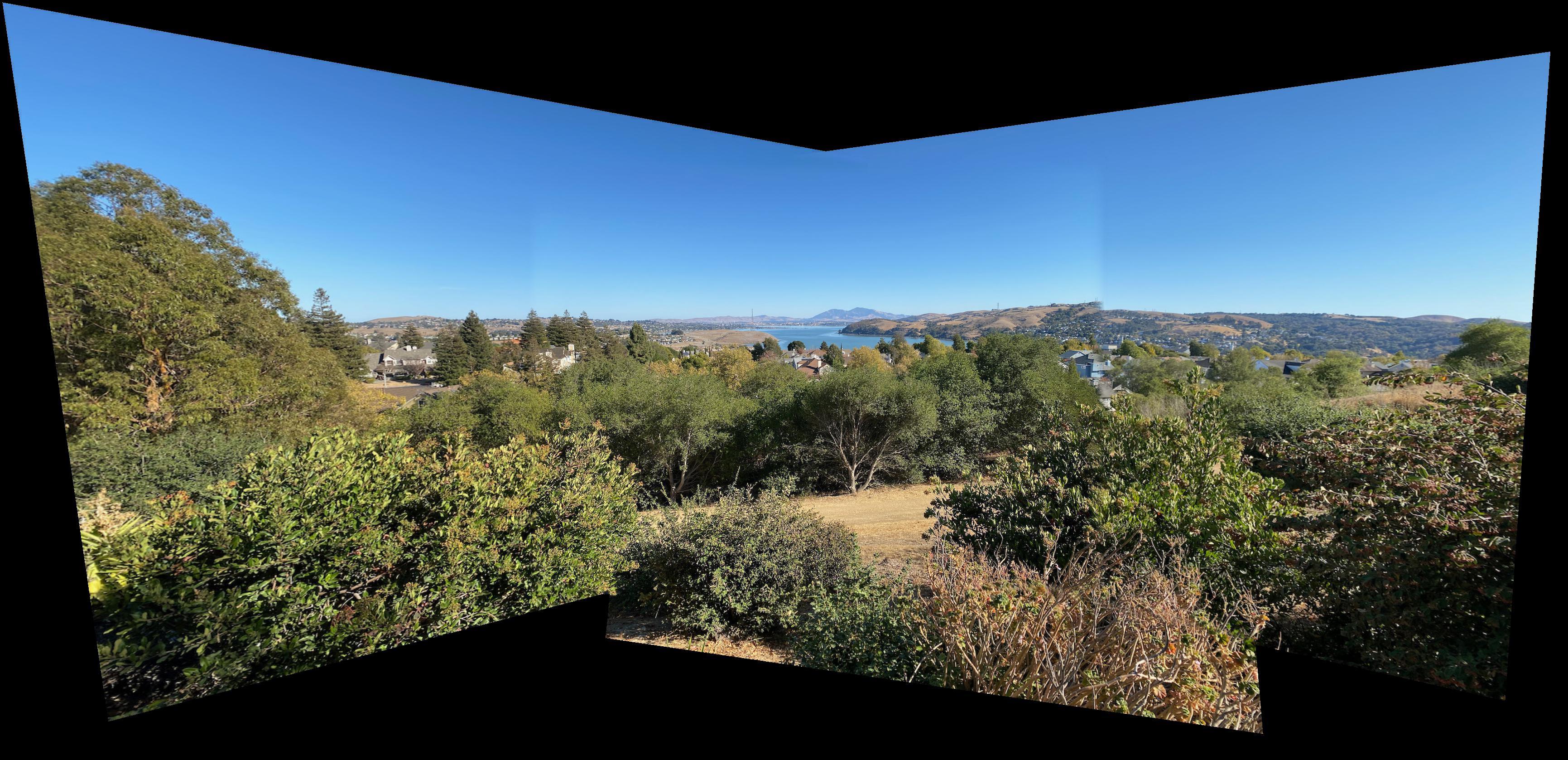
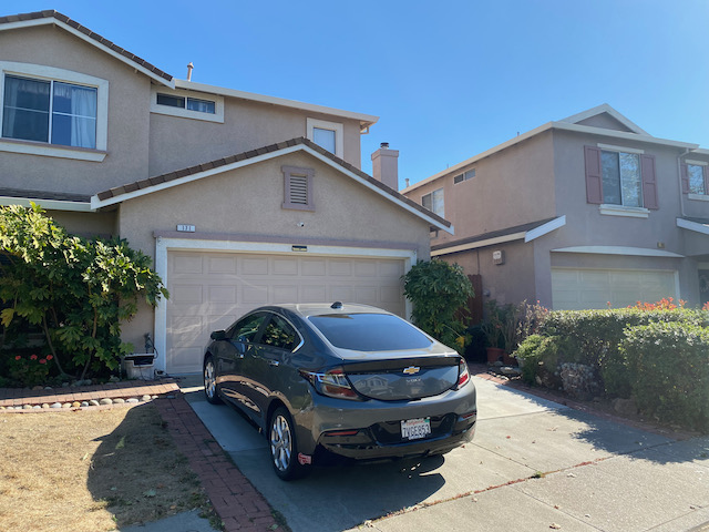
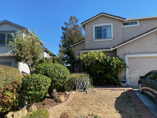
House Exterior
| Source Images |
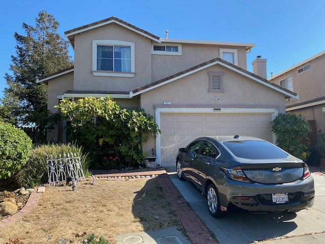 |
 |
 |
| Manual (Part A) |
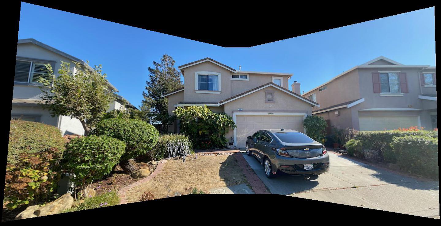 |
| Automatic (Part B) |
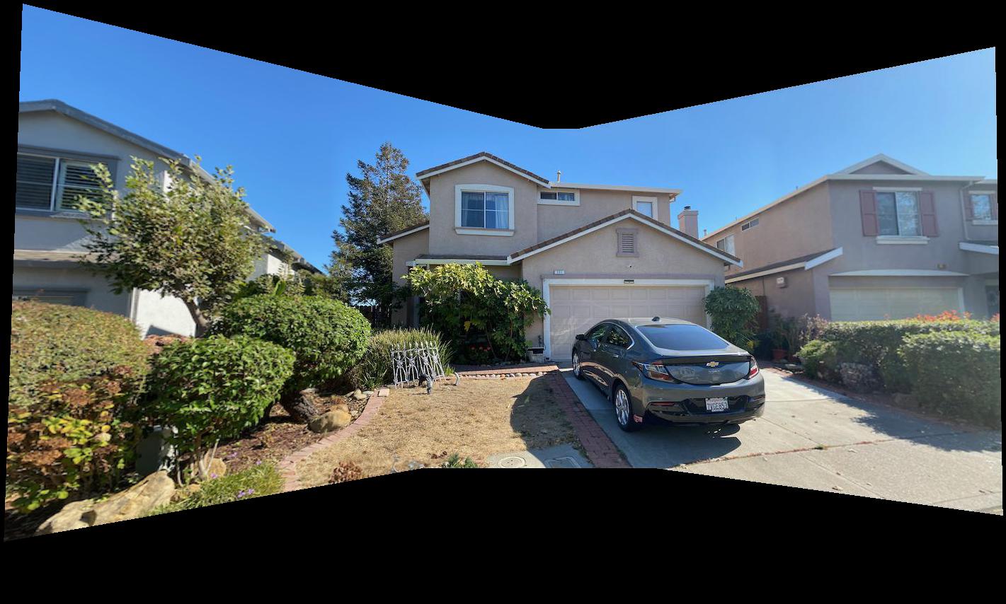 |
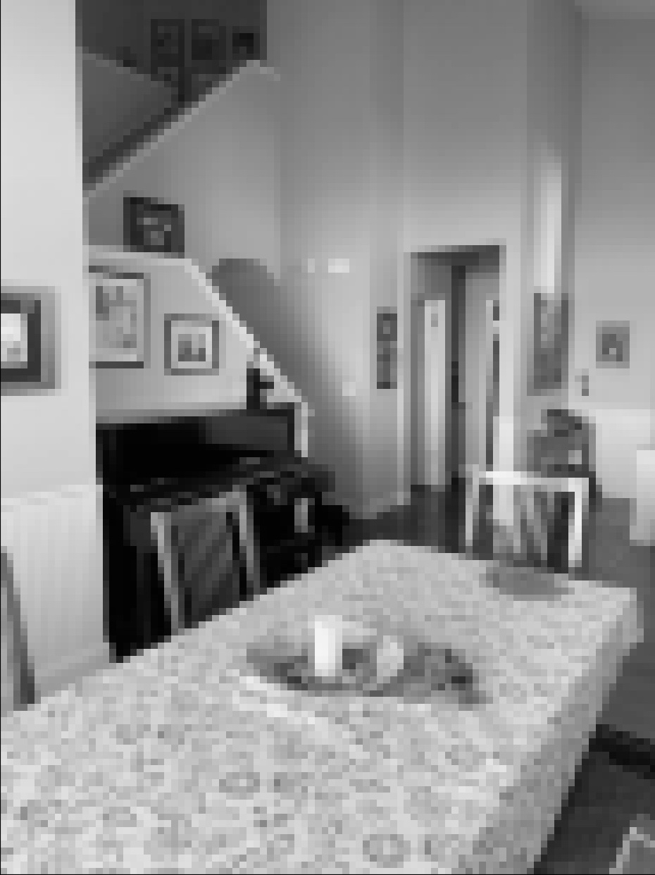
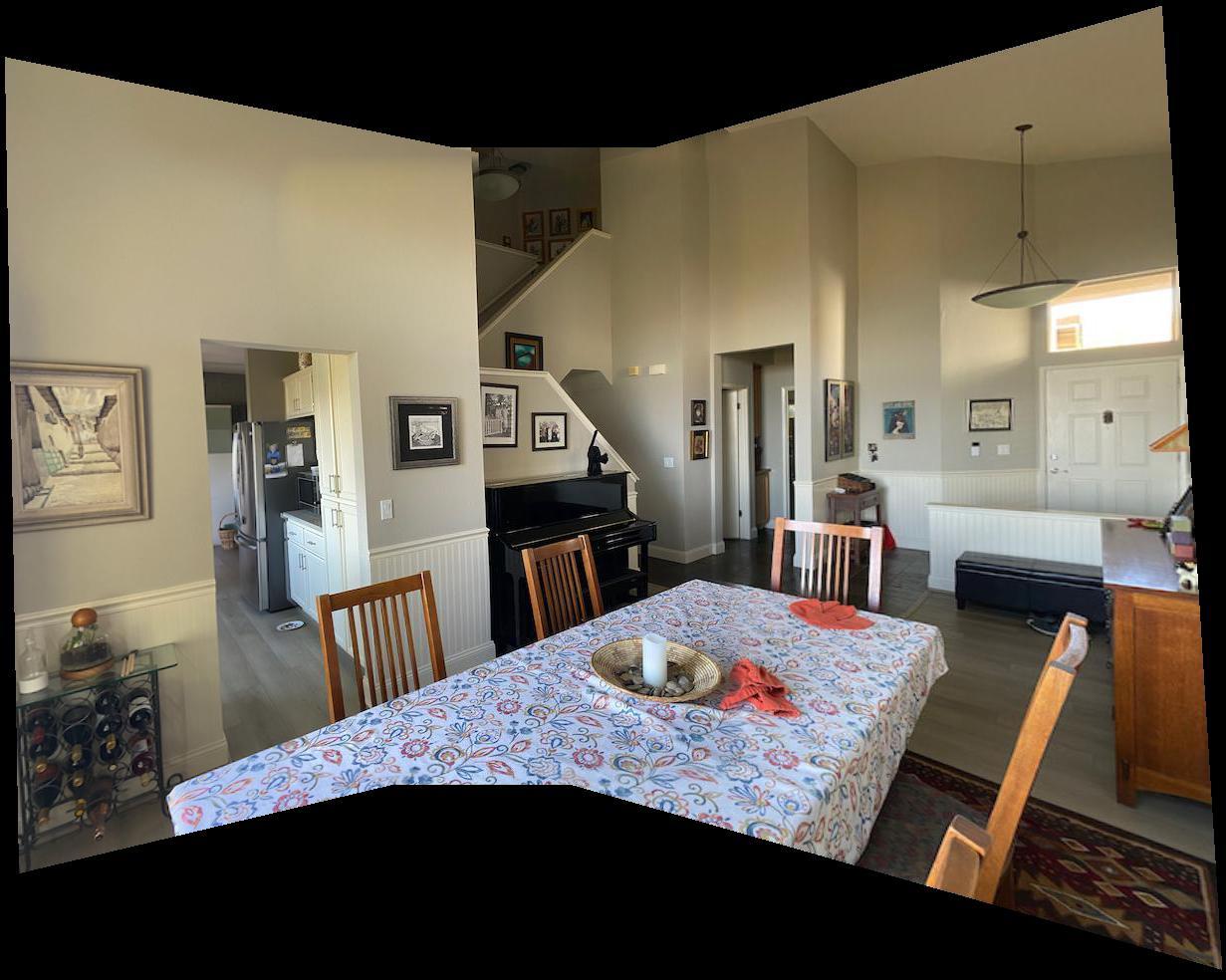
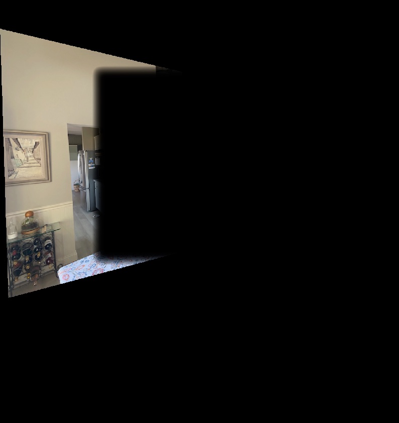
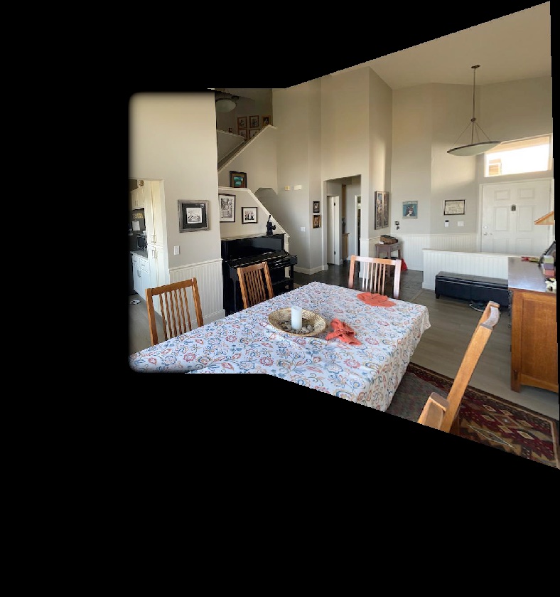
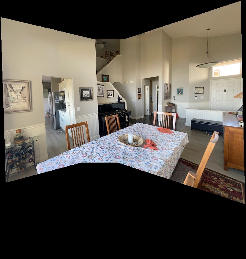
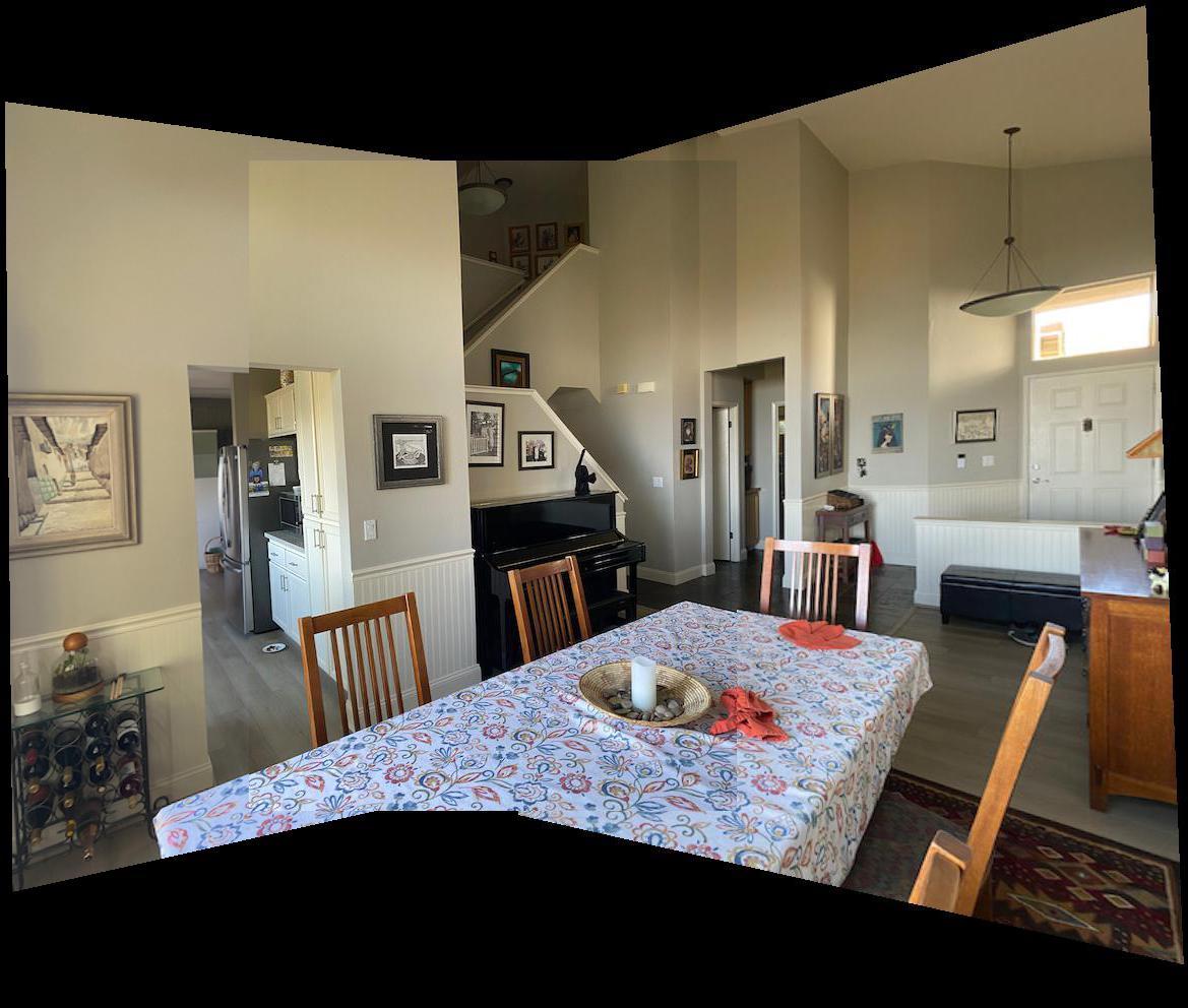
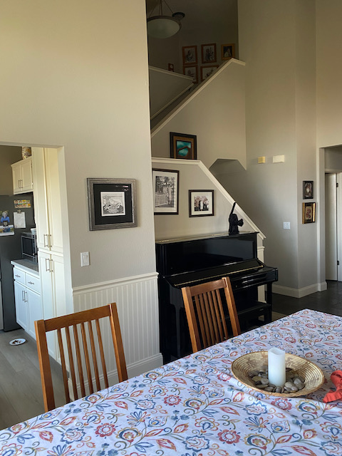
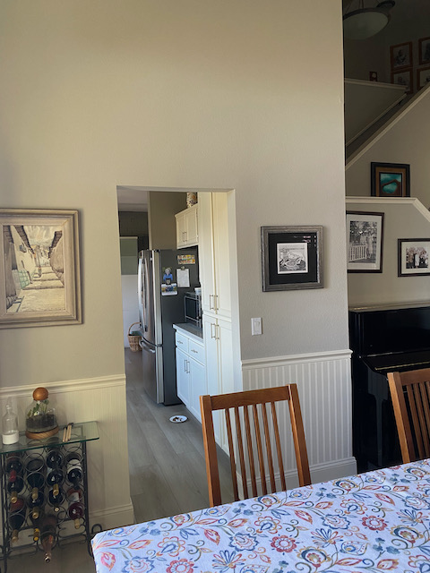
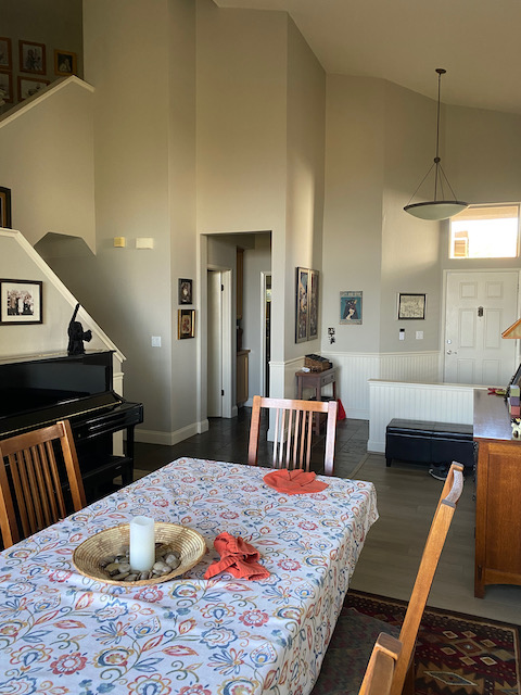
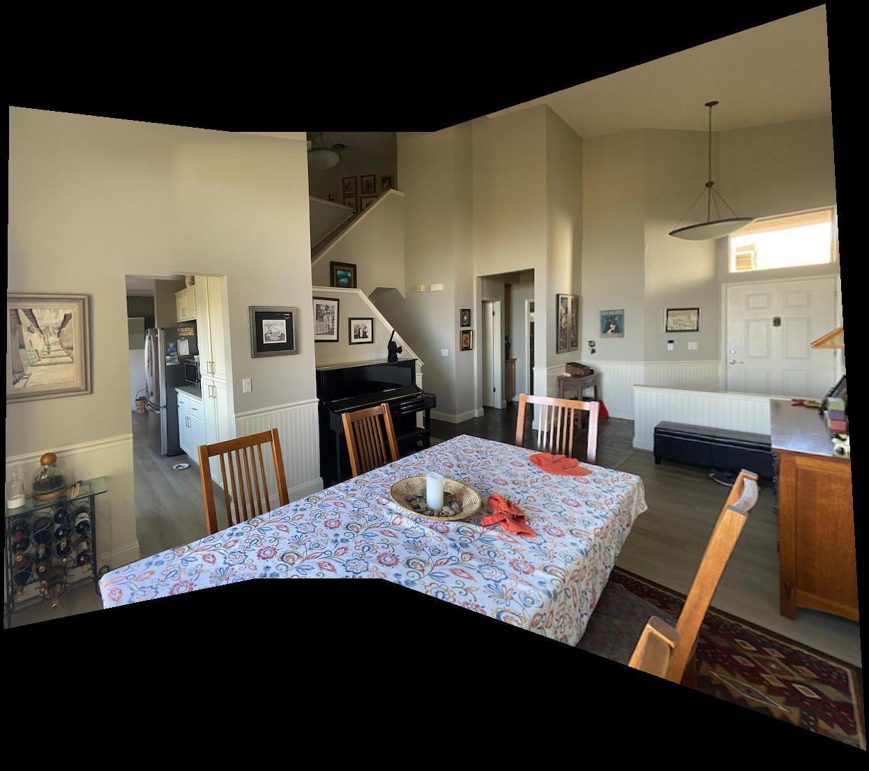
House Interior
| Source Images |
 |
 |
 |
| Manual (Part A) |
|
| Automatic (Part B) |
 |