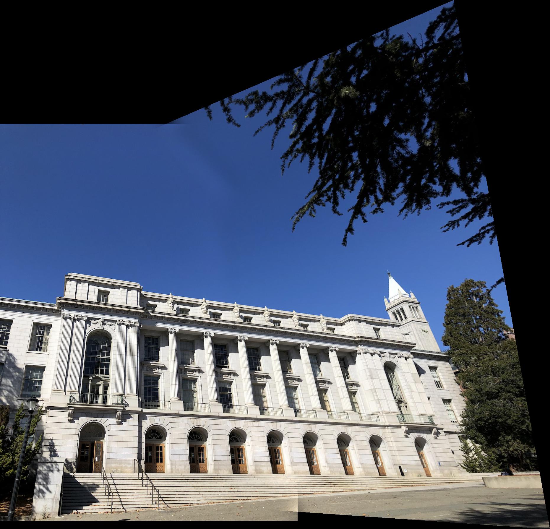
In this project, I used projective warping to rectify images and blend multiple images together in to a mosaic/panorama.
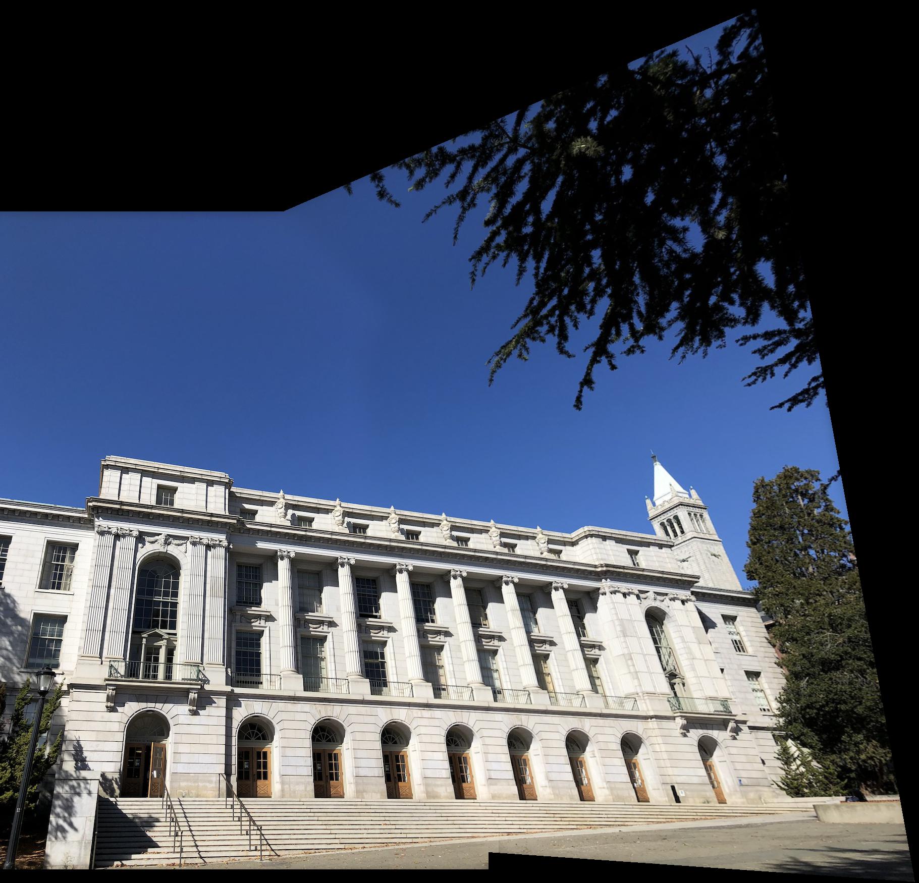
I shot the photos on my smartphone camera and transferred them to my computer. I tried to rotate my camera while avoding translation when shooting the photos for the mosaic. I also used the AE/AF lock feature on iOS to keep the lighting consistent.
We first have to compute the homography matrix H that defines the warp.
Next, we can solve for x' and y' by dividing wx' and wy' by w
Finally we can format the equations as a matrix, and use least squares to solve for the optimal [a b c ...] vector.
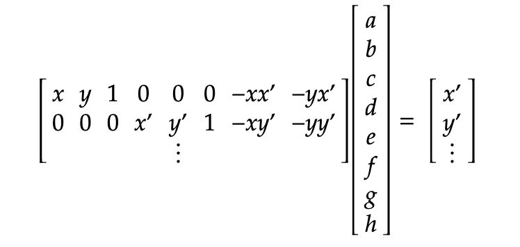
I used np.linalg.lstsq to find h and then reshaped it in to a 3x3 matrix. The minimum number of points needed is 4, but it is good to select more points for a more stable solution.
I then wrote the function warpImage to warp an image with the matrix H. I use H to calculate the new bounding box of the image, and the inverse of H to sample the pixels with interpn. My implementation can either compute the warped image dimensions automatically, or work with a fixed canvas. The image returned by the function also has an alpha channel so it is easy to disntiguish the image from the blank background.
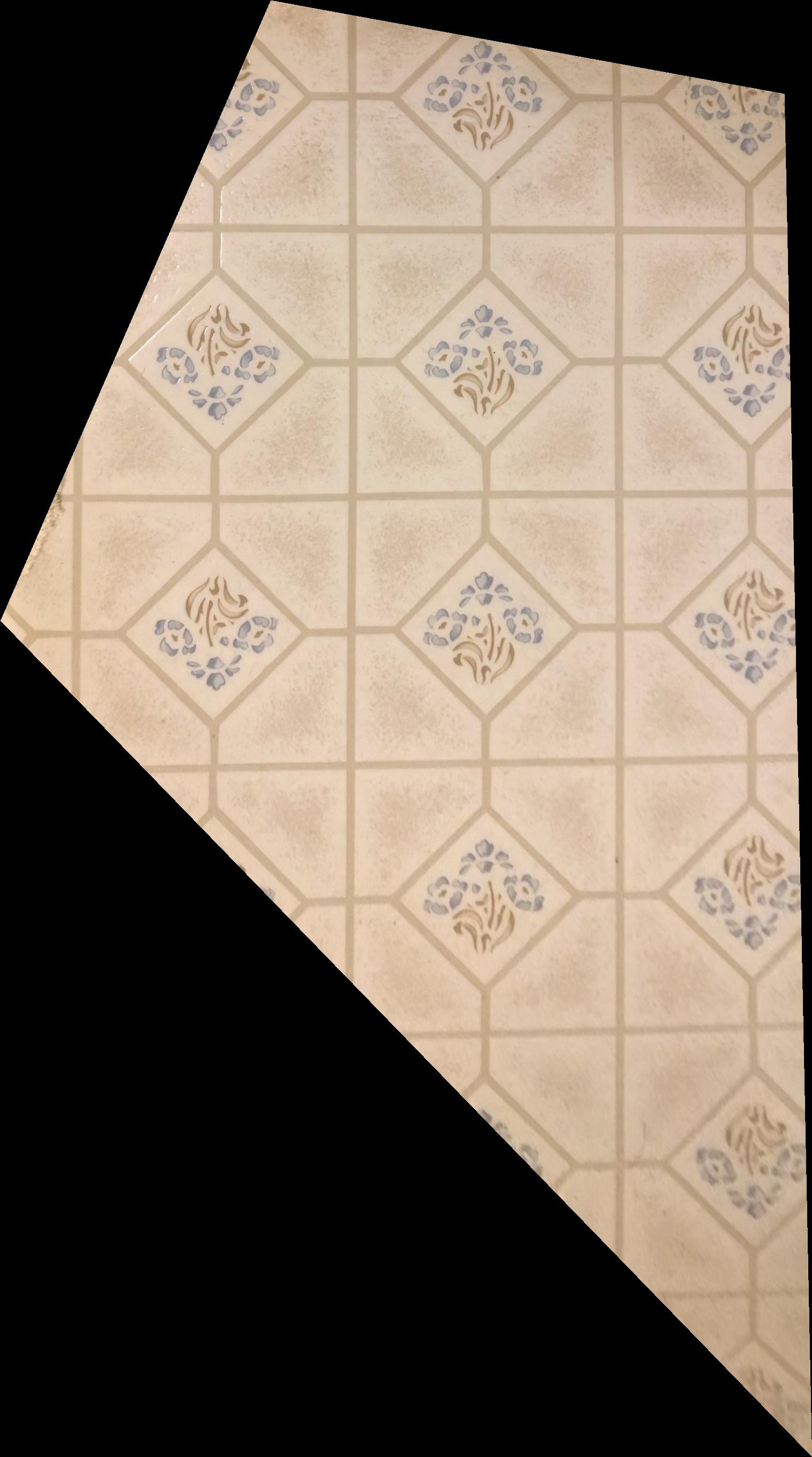
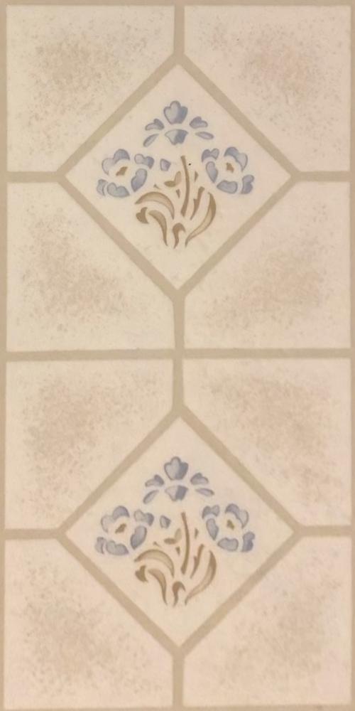
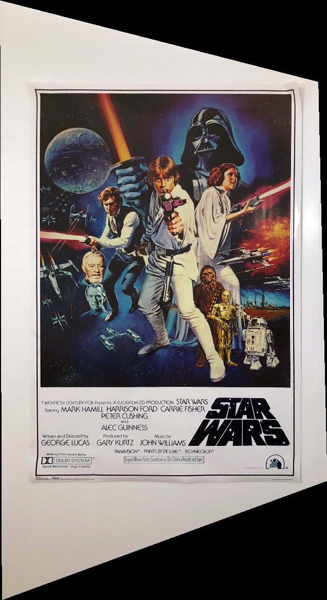
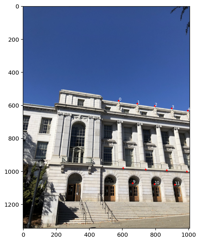
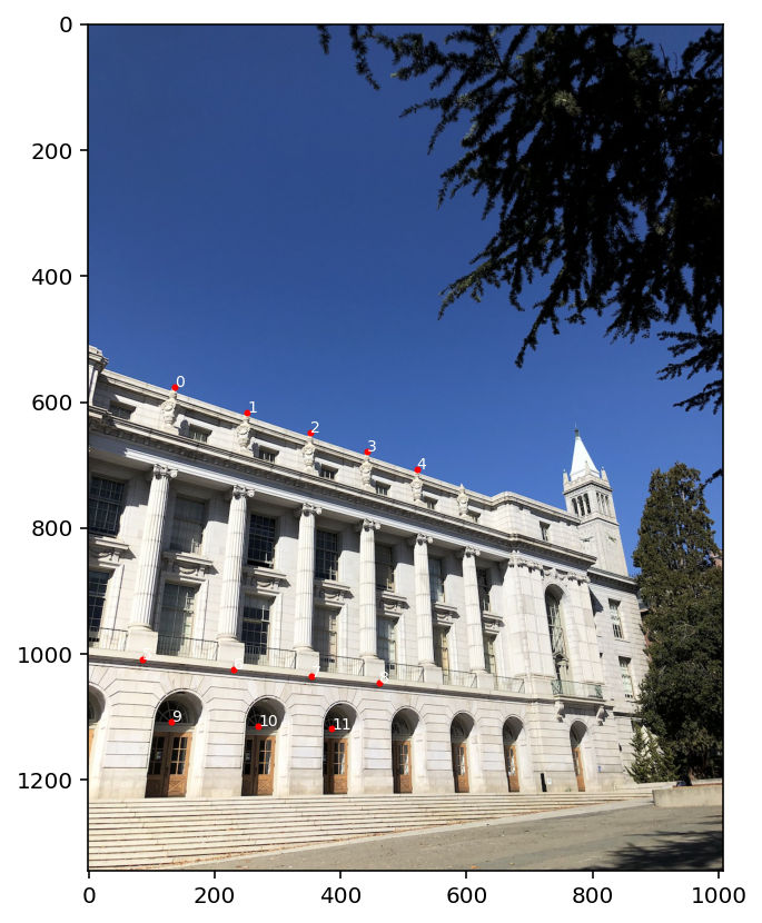
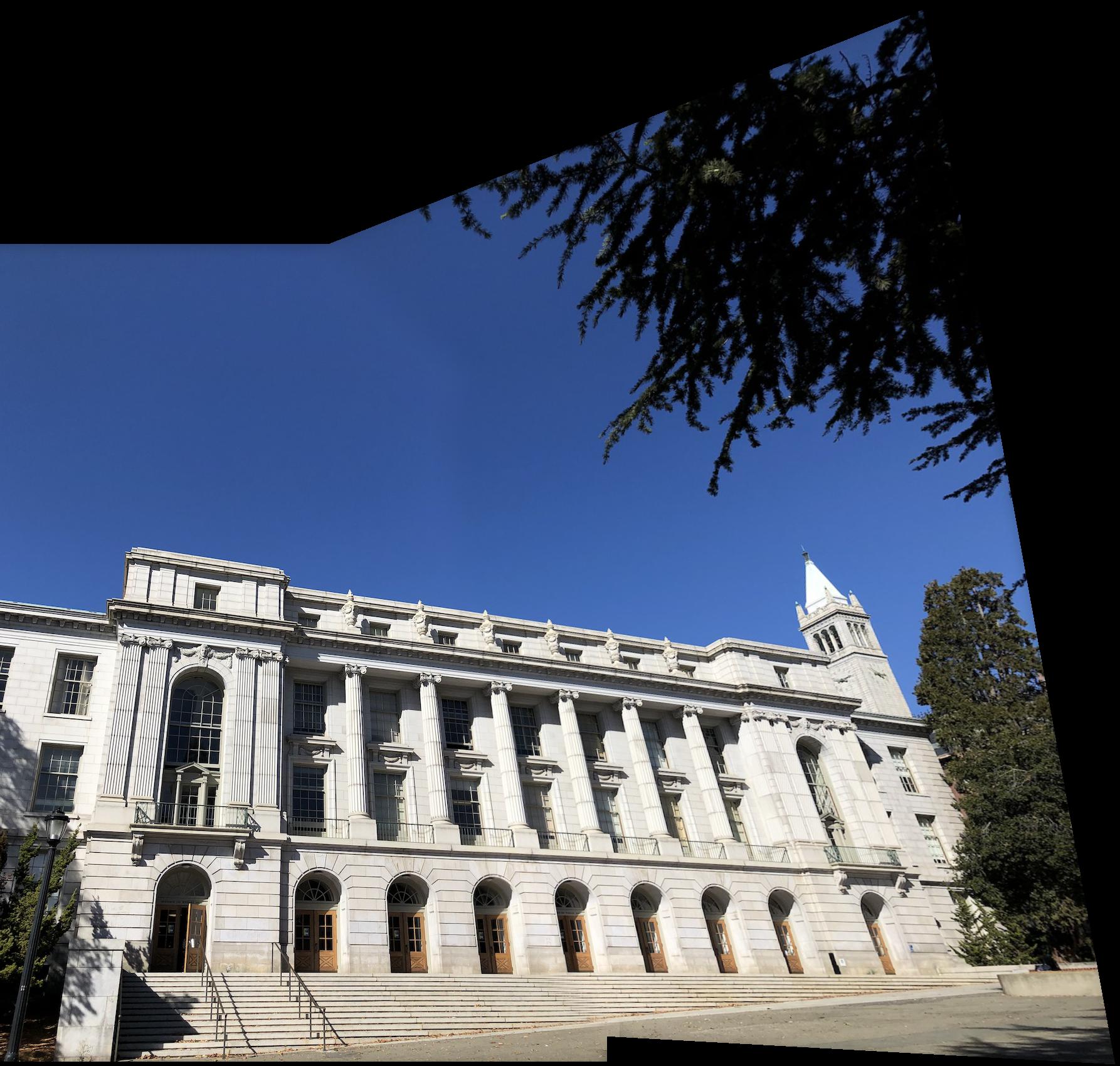
Image rectification means transforming a picture of a planar surface so that the plane squarely faces camera. I defined points at the corners of the plane I wanted to rectify, and computed the transform to make the corners form a rectangle.
|
|
|
|
|
|
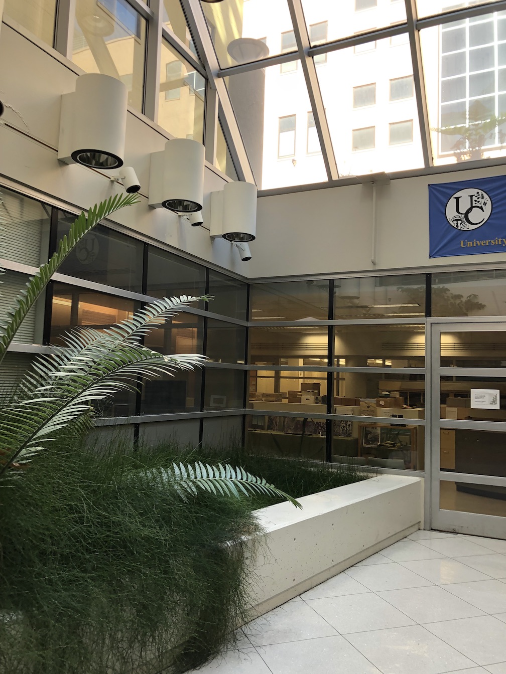
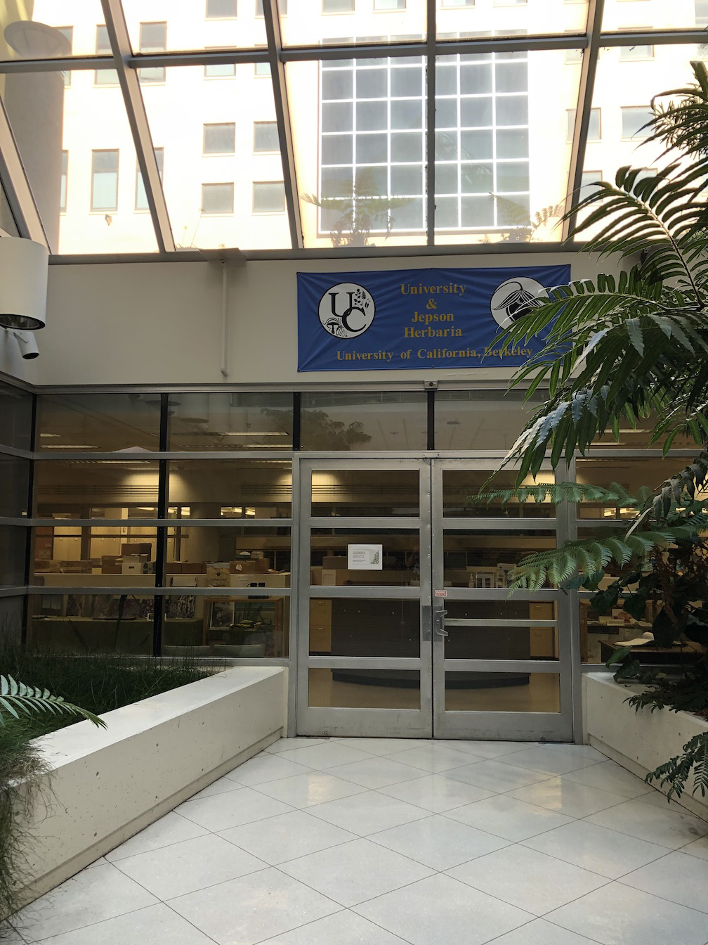
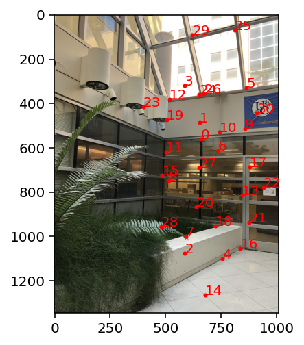
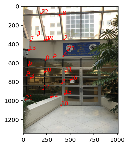
To blend multiple images together, we first have to define correspondences between matching keypoints. In the image below, I hand selected points at easy to identify corner locations that were present in both images.
|
|
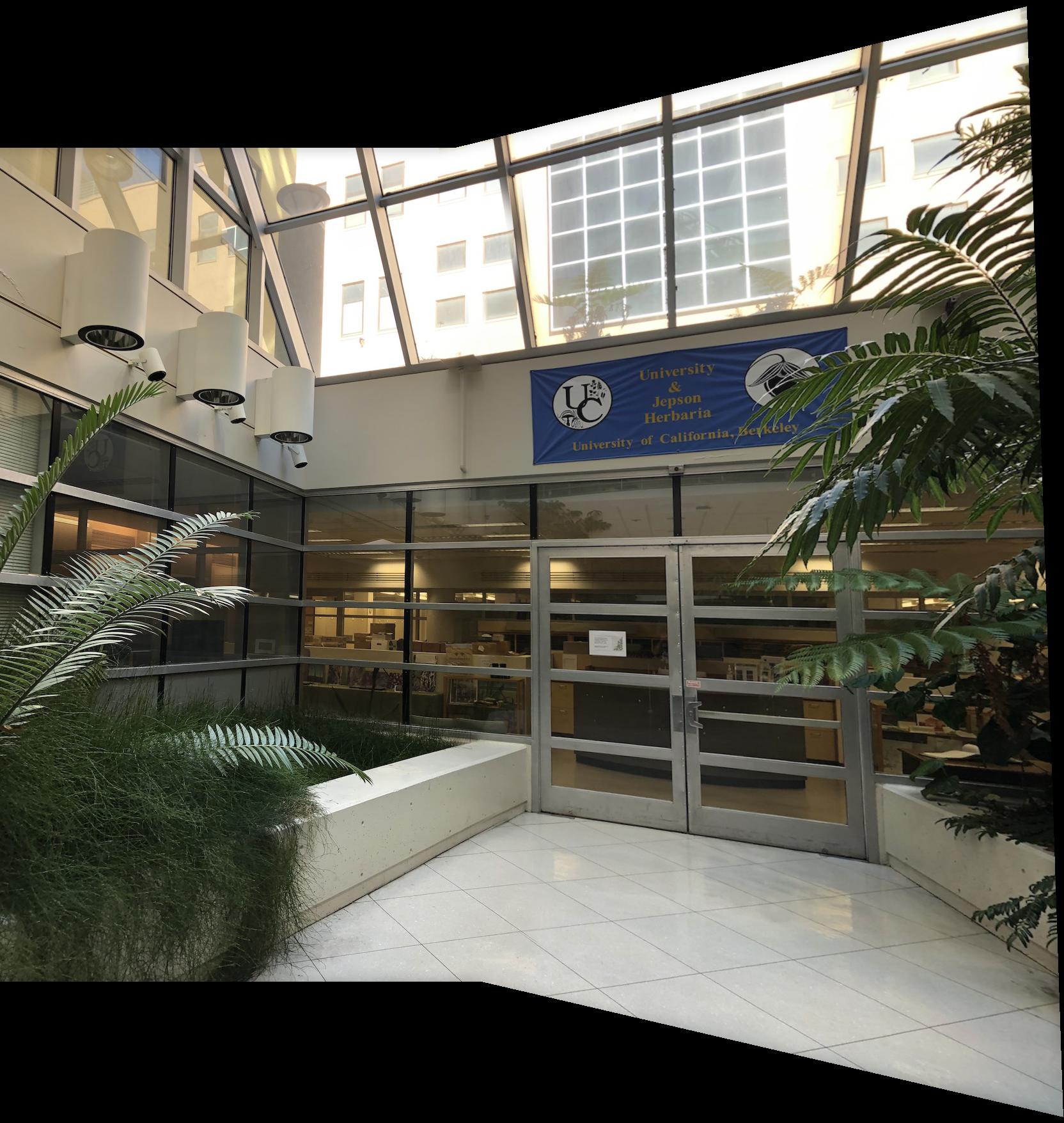
I then warped Image B so that its points lined up with the points on Image A. I initially used alpha-weighting to blend the images (in areas where the image overlapped, I took the average of the two pixels at the location)
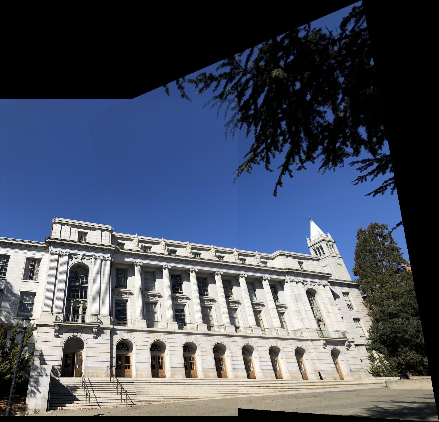
Because of differences in exposure, you can see a pretty clear seam in the image, and the left side of the tree at the top-right of the image is faded. In addition, if the images are not perfectly aligned or taken from the same location, then there will be ghosting/blurriness in the overlapping sections if alpha-weighting is used.
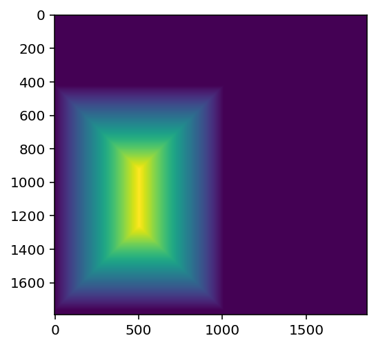
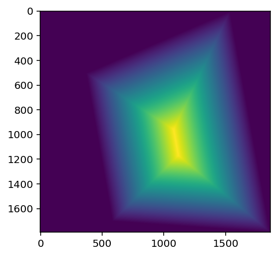
A more advanced strategy is to blend based on a distance function. I used scipy.ndimage.distance_transform_cdt, which sets the pixel value to the distance to the nearest image edge.
|
|
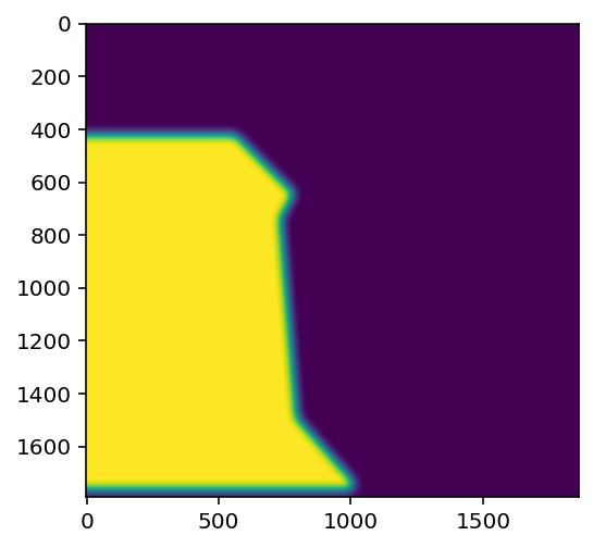
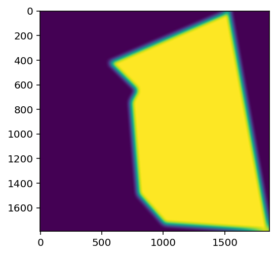
Using these distance functions, I created a mask for each image based on if the image has the maximum dist value at the point. For image A, the mask is (distA > distB). I also added a gaussian blur so the transition isn't as harsh.
|
|
When I blend the images with these masks, there is a bit of ghosting at the edges because of the blur. Using the distance function (which we already have), I inset the image by a fixed amount to crop out the blurry parts. The result in the cropped image is nice with no ghosting and the seam is nearly invisible.

|
|
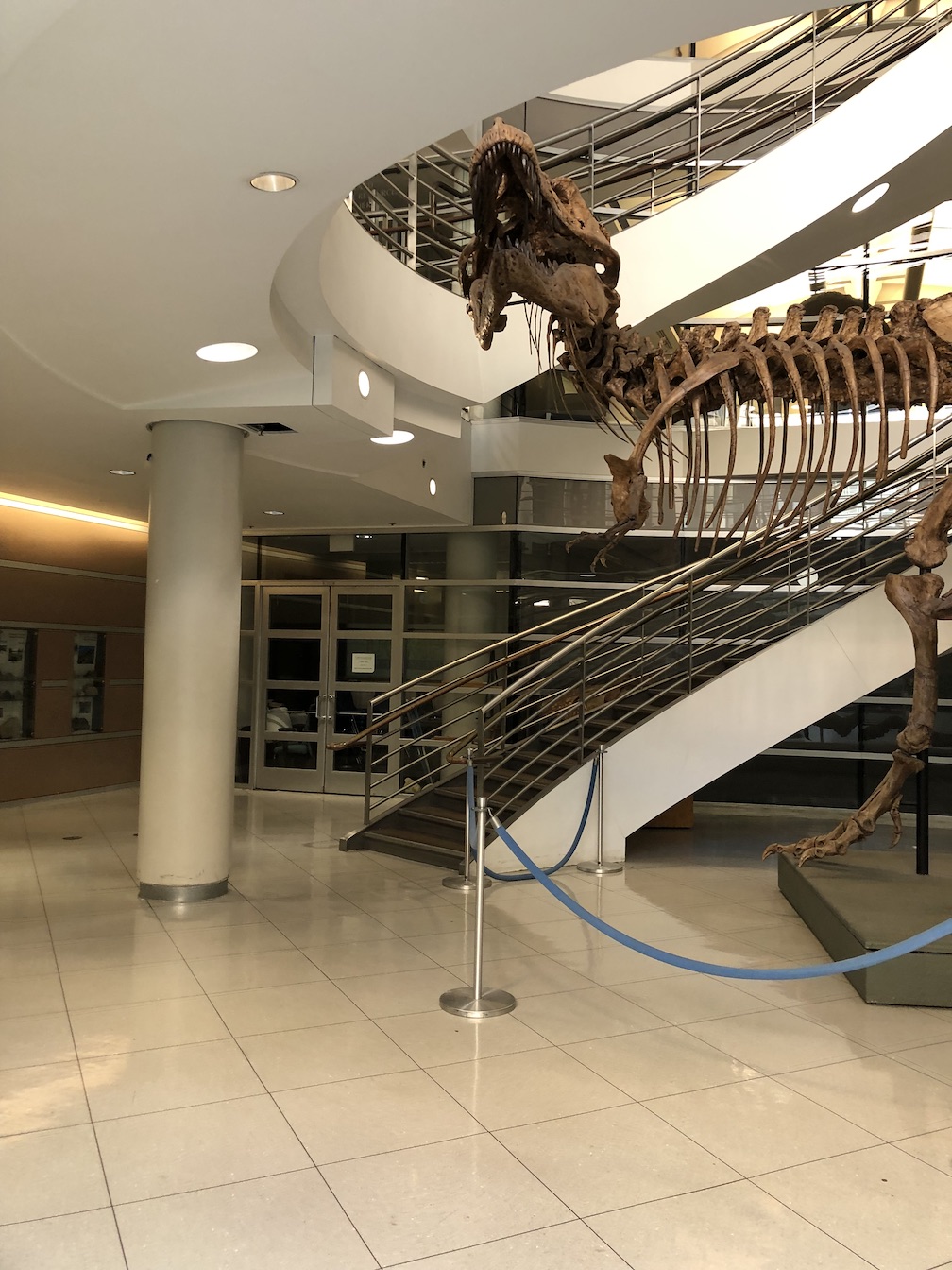
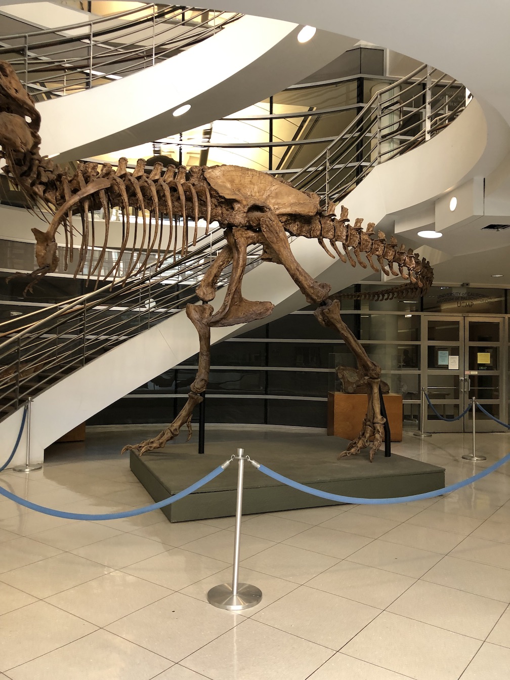
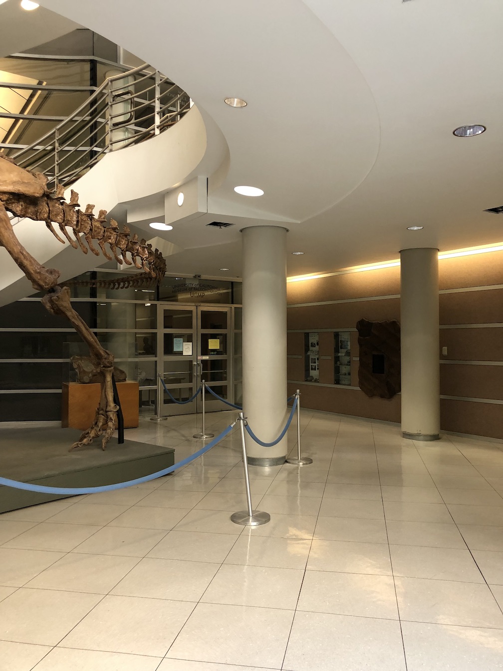
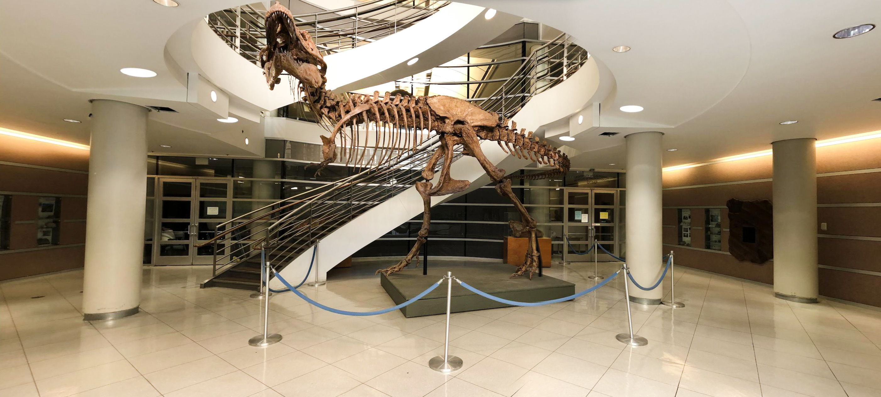
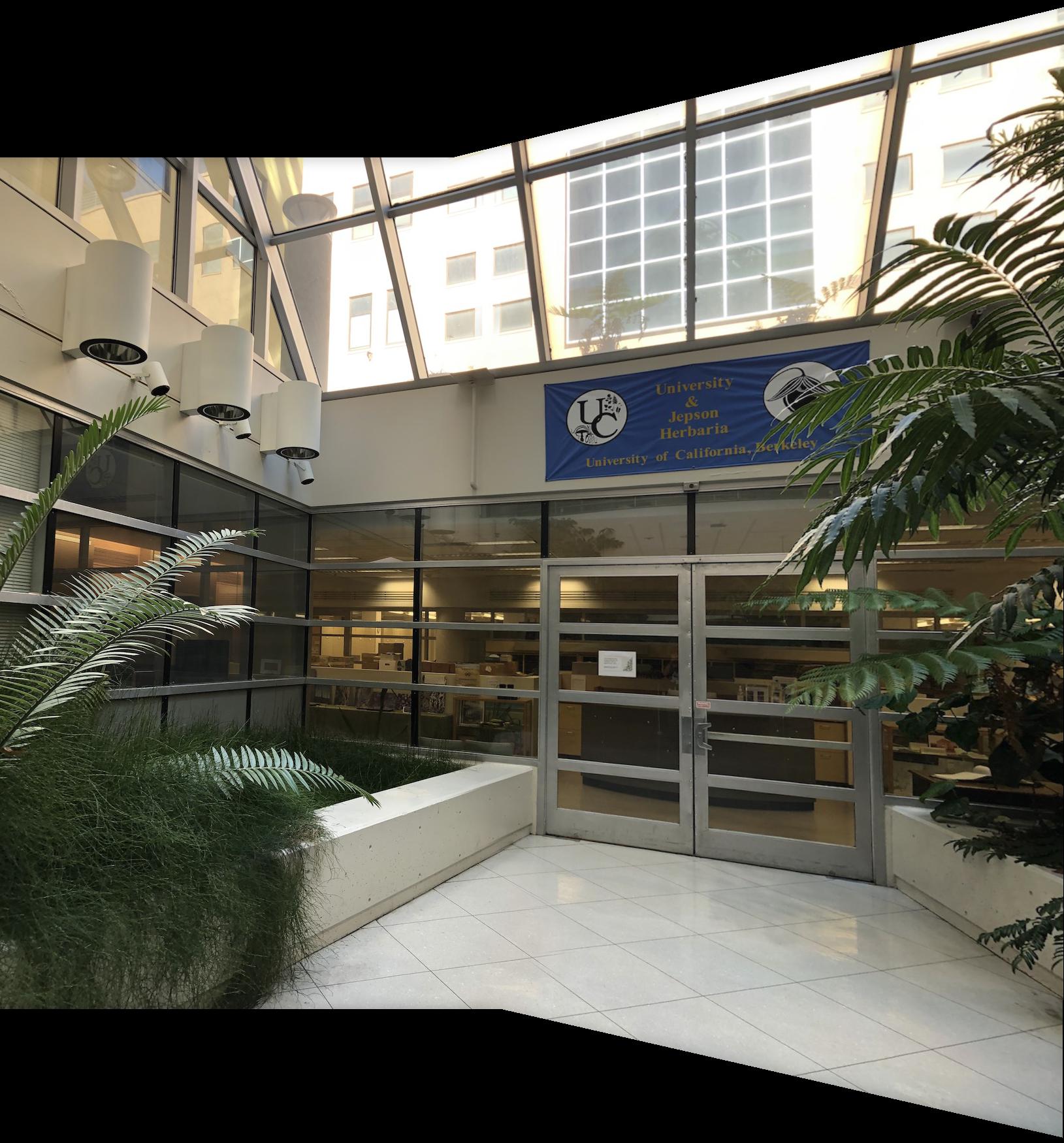
Here are a few more mosaics I made:
|
|
|
|
|
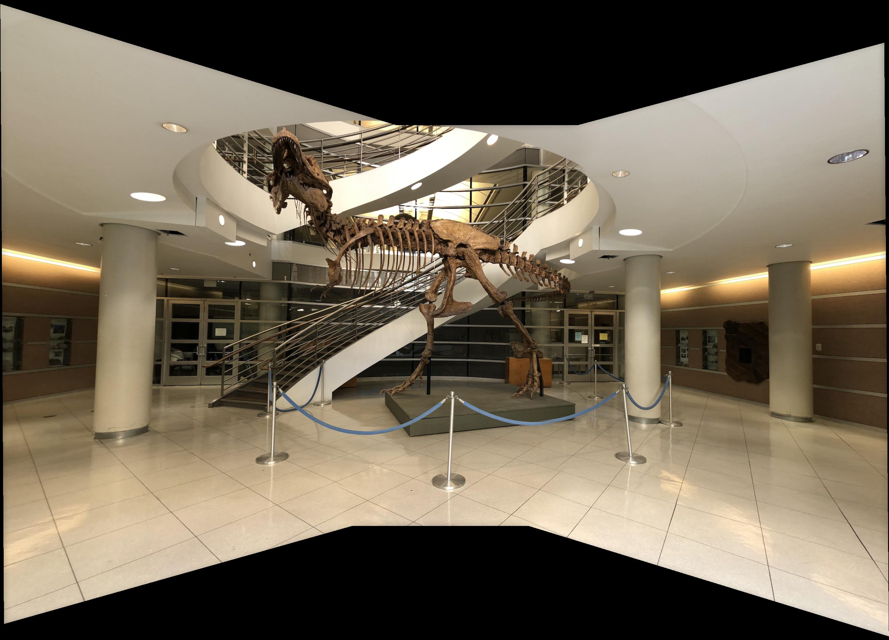
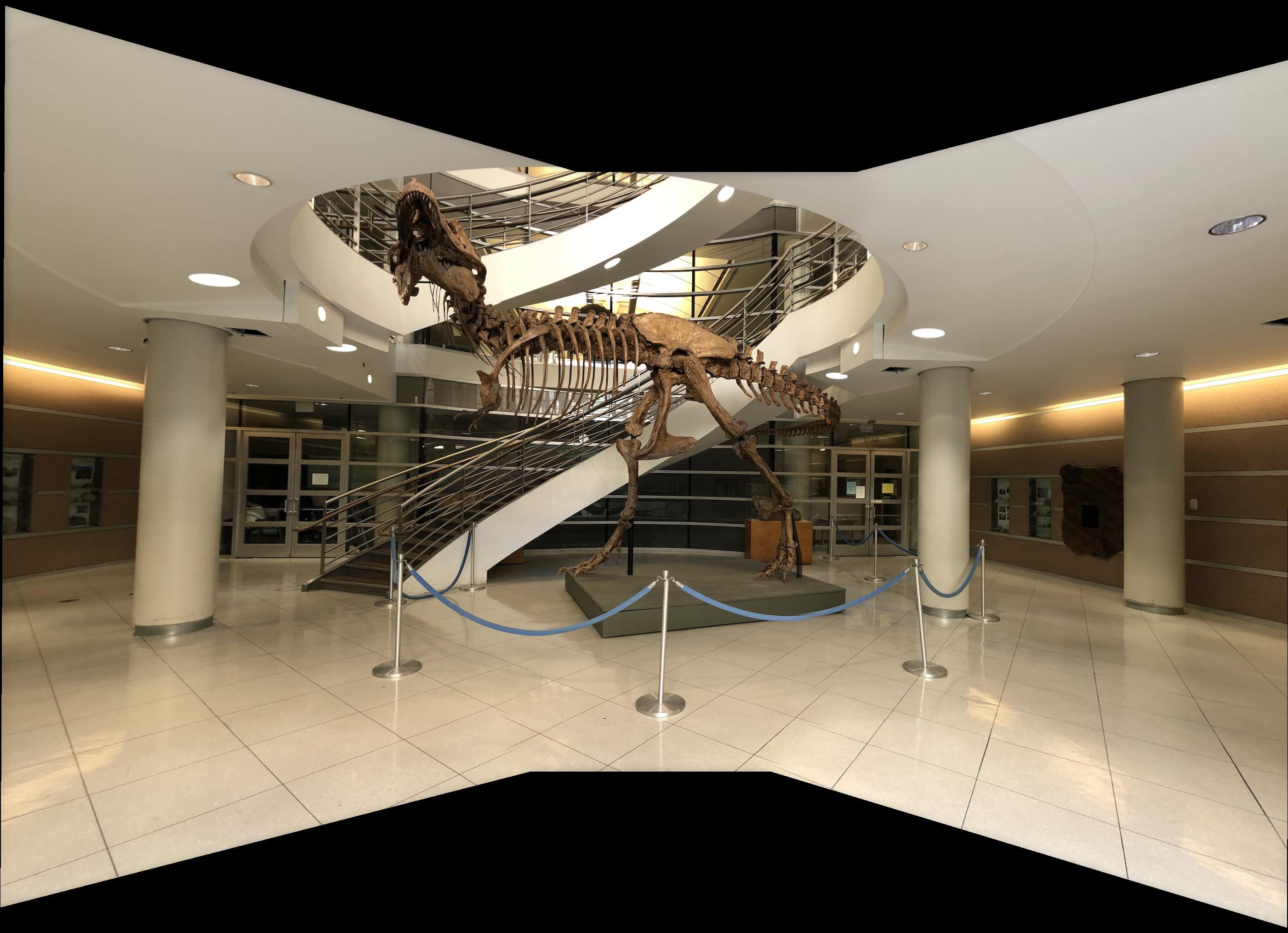
With a bit of cropping and lighting adjustments in Photoshop/Lightroom, I can get a pretty clean looking result (shown below). The T-Rex's name is Osborn, btw.
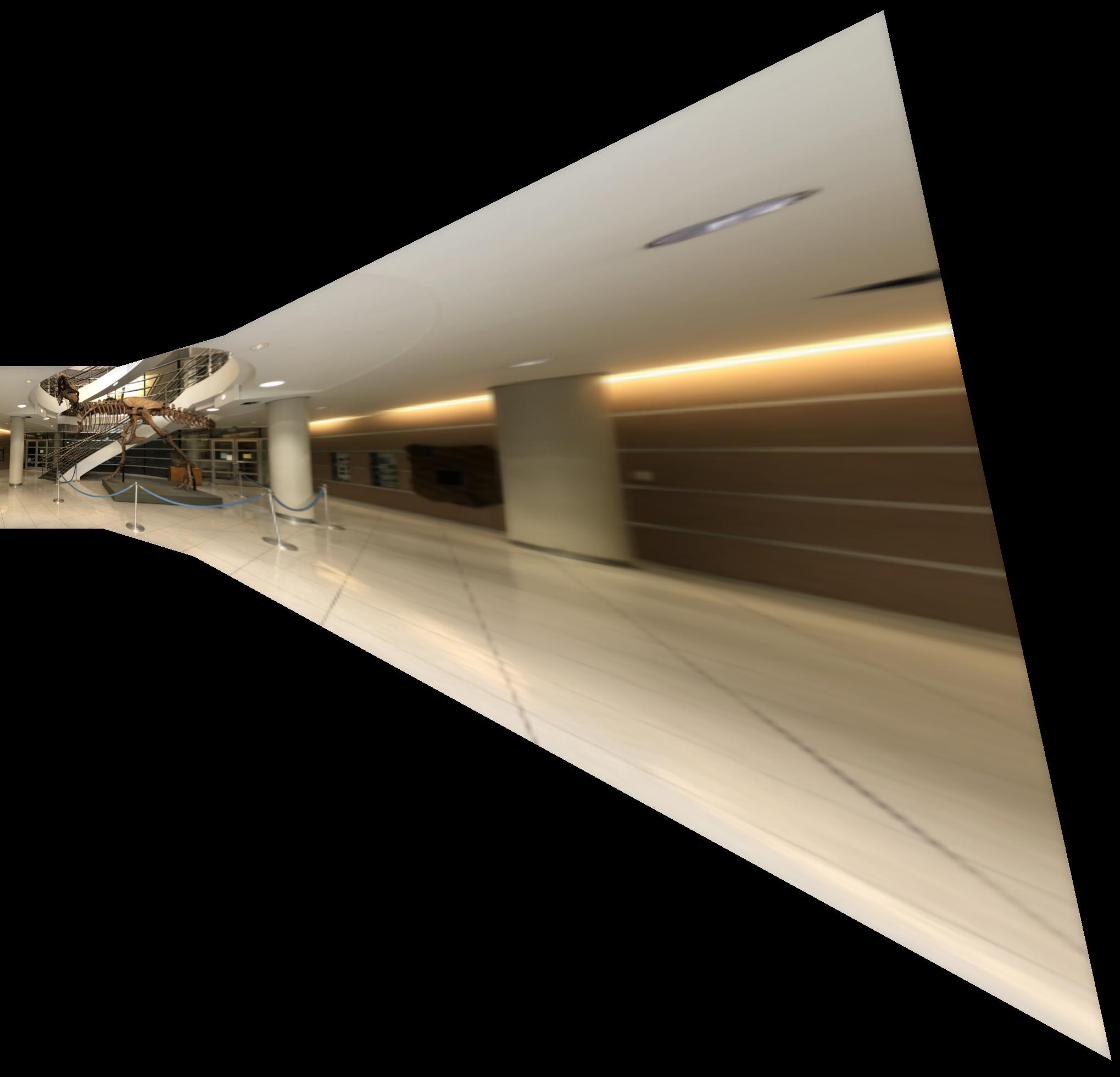
My mosaic blending code automatically finds the canvas size and also supports cases where transformations are chained (In the image below, the left image is fixed, the middle image is warped, and the right image is transformed to the warped version of the middle)
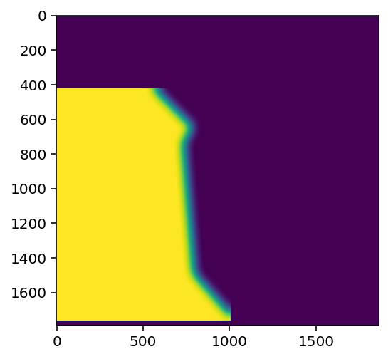
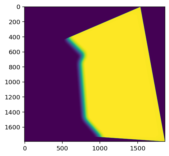
I tried creating improved image masks for blending that were blurred at the intersections with other images, but not blurred at the borders of the mosaic. I did this by transforming the masks from canvas space back to the coordinate space of the original image, blurring them (taking advantage of the symmetrical boundary mode in scipy.signal.convolve2d), and then transforming the masks back to canvas space.
|
|
Because the border edges are now hard, there is no need to crop and I can use the entirety of the image.
|
|
With advanced blending, the border edges are hard, while in regular blending the border edges are ghosted. The drawback is that the seam of advanced blending is not as good.
I thought learning the way we set up the least squares problem for finding the homography matrix was pretty interesting. This was also my first time seeing the distance transform and I thought the application for masking was clever.
In part B, we create a system for automatically stitching images together.
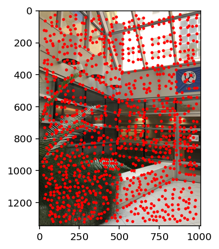
I used the provided method to get the harris corners, and then implemented Adaptive Non-Maximal Suppression to get spaced out points. In a nutshell, the surpression algorithm picks features that are far away/isolated from other features bigger than themselves.
I set c_robust = 0.9 as recommended by the paper, and picked the points with the 100 largest radius values
|
|
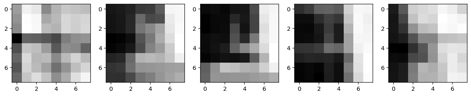
I extracted a 40x40 feature patch for each point, and downscaled it to a bias gain normalized 8x8 feature descriptor (setting the mean to 0 and the stddev to 1). Here are some example patches (with just the R channel so they are not clipped).
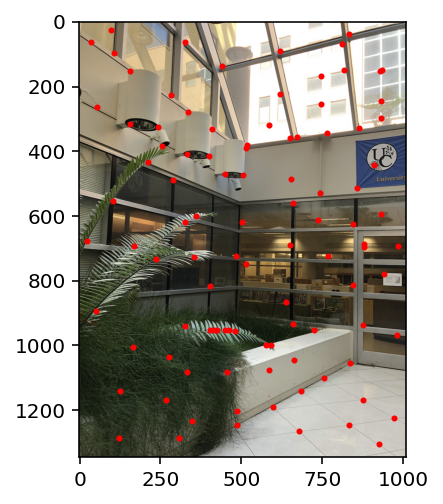
I used Lowe's thresholding to find features that matched. I measured distances based on SSD and picked matches where (1-NN/2-NN) < 0.5.
|

|
Incorrect matches include point 23 on the lamps, and point 4 on the floor corner.
I implemented RANSAC to filter out the bad matches. In each loop, I select four pairs, compute H using just those 4 pairs, and count the number of inliers (pairs whose coordinates are close together after one side is transformed with H). I pick the iteration with the largest number of inliers, and run least squares on all the inlier pairs to compute the final H.

|
|
Thanks to RANSAC, the incorrect matches in the image above are now gone.
| Auto | Manual |
|
|
|
|
|
|
I learned how the Adaptive Non-Maximal Suppression worked from reading the paper, and how in general to read a research paper.