Overview
In Part A of this project, we aim to compute homographies between image planes and use this to create mosaics.
Part A1: Shoot and Digitize Images
|
|
|
|
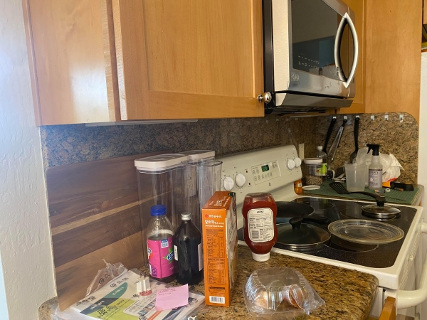
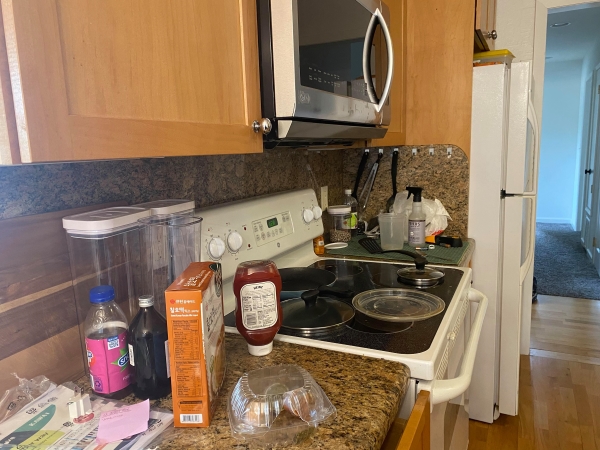
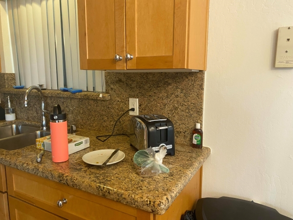
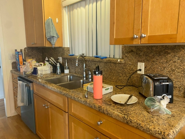
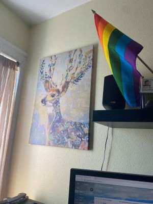
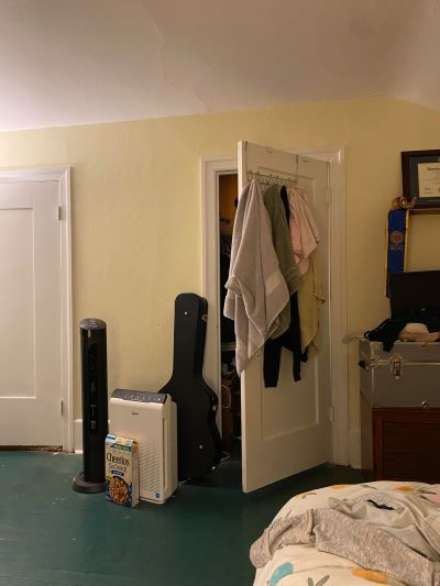
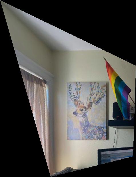
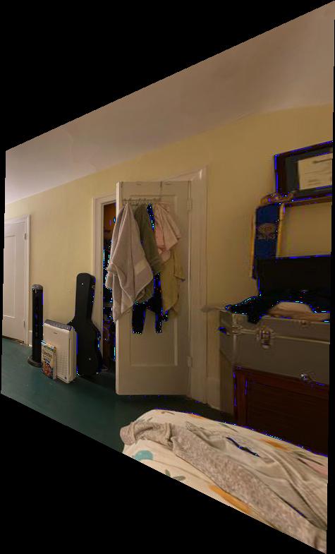
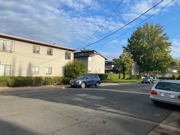
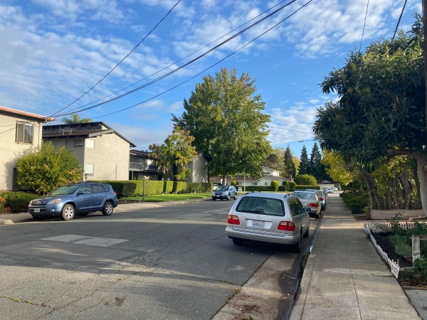
For the following parts of the project to work (particularly the mosaicing), it is important for us to take photos that have the same center of view. For this project, I used my smartphone (iPhone 11) and tried to rotate my body while keeping the camera still. I locked the exposure and focus to make sure the photo looks consistent. The above are the photos for the mosaic. The below are photos used to show image rectification.
However, you will note in Part 5 that this technique was probably insufficient for photos this close up. The fact that the photos are taken close up and without a tripod means the center of projection was not the same between photos. This means the homographies will not achieve perfect results.
|
|
Part A2: Recover Homographies
|
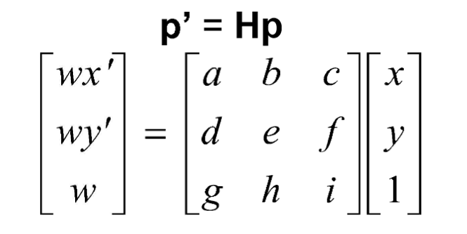
To properly warp the images, we must first recover the homography to do so. Figure 3 shows how the homography is set up. We are looking for the values of H. We know wx', wy', x, and y. wx' and wy' are the target coordinates in a plane. The x, y are the source coordinates from the originaly image. We set i to be 1, and we then try to solve for the remaining 8 parameters a-h.
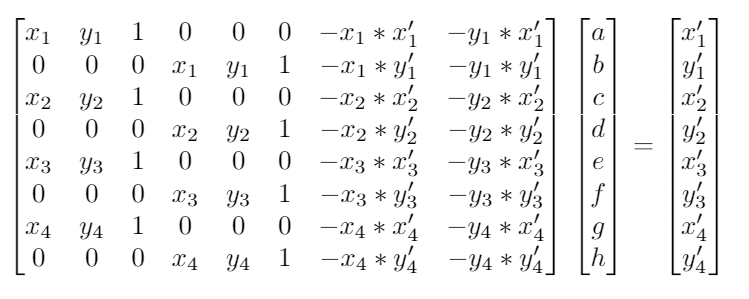
To do so, we can set up a system of linear equations. We primarily note that wx' = ax + by + c. wy' = dx + ey + f. w = gx + yh + 1. Rearranging all this gives us the following system of equations:
|
Once in this form, we can solve for the entries a-h. However, we can also extend this to be an overparameterized problem. Rather than include only 4 points, we can extend this to any n points instead. This means that the H matrix is n*2 rows by 8 columns. The corresponding b matrix is n*2 rows as well with x and ys alternating. We can solve this with a linear least squares solver such as numpy.linalg.lstsq.
Consequently, we can quite easily define a function computeH(im1_pts, im2_pts). im1_pts contains all the x, y to populate the A matrix. The im2_pts contains the x', y' to populate the b matrix. Then we use linear least squares to solve for elements a-h and use 1 to round out the 9th value. This is our homography matrix.
Part A3: Warp Images
Once we have the homography, we can write some function warpImage(im, H) that warps the image to the desired plane. We use inverse warping. We do the following steps.
- Calculate where all the corners of the image go in the new plane. Use this to calculate the shape of the bounding box for the warped image.
- Calculate where all the internal pixels go. This is actually done with an inverse warp.
- Calculate H_inv
- Multiply H_inv with every pixel in the new image that corresponds to pixels from the source image.
- Now populate the colors properly.
- Generate the RectBivariateSpline functions for each color channel of the image
- Use these functions to inverse warp to get the appropriate colors.
This is very similar to the warping that we did in the previous project.
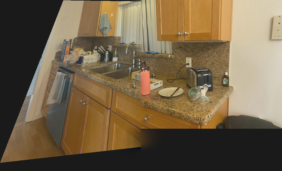
Part A4: Image Rectification
Now that we have the warp, we can "rectify" images. In these examples, we take images of planar surfaces and then warp them so the plane is frontal-parallel. We find the pixels of the corners of our planes, decide where we want them to go in the final image, and then call computeH and imwarped accordingly to generate the following images.
|
|
|
|
|
|
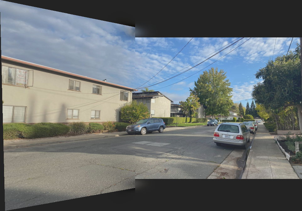
Part A5: Mosaics
For this part, we blend 2+ images into a mosaic smoothly without edge artifacts. To do this, we defined correspondence points between the images. We then used these correspondences to compute some homography H between the images to warp one into the other using from the previous prats. We then used Laplacian blending from Project 2 to smoothen out the edges.
|
Two of my scenes were indoor scenes, shown below. These photos were taken with a cell phone camera and without a tripod. As such, the center of projection for the images are not the same. Additionally, I suspect there is some distortion on the edges of the camera. However, primarily because the photos were taken up close and without a tripod (not the same center of projection), even with 20+ correspondences, the homographies cannot get the whole image to line up properly. As such, there is some disconnect between the complete images.
|
|
|
|
|
|
|
|
You can note that Figure 8C is substantially worse than Figure 7C (ie: it looks more like you're seeing double). 7A and 7B were taken more steadily than 8A and 8B. The change in the center of projection is worse in 8A and 8B, eventhough the images are roughly similarly far away.
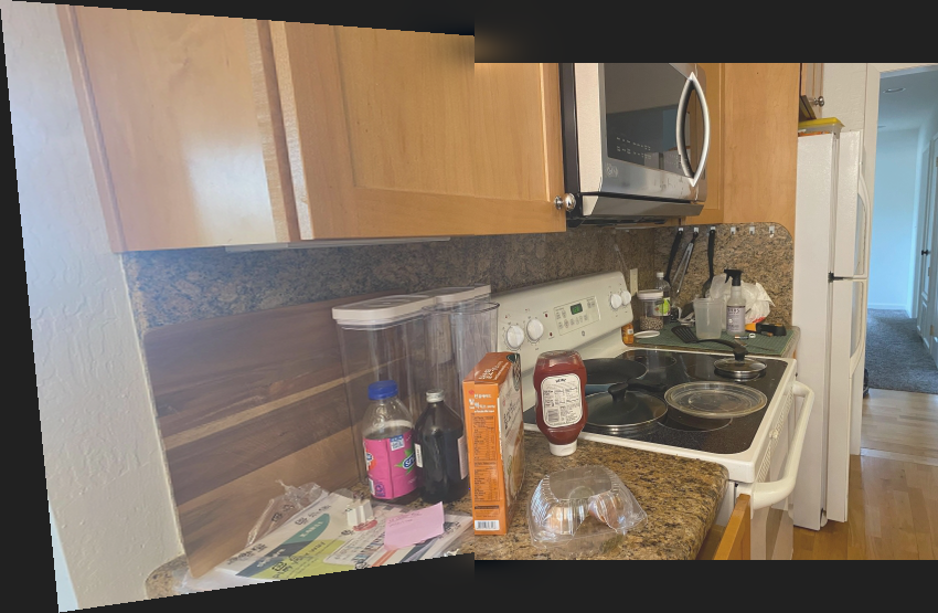
However, you can note that for the next mosaic, the photos were taken of things that are roughly far away. Because of this, the resulting mosaic is much more lined up.
|
|
|
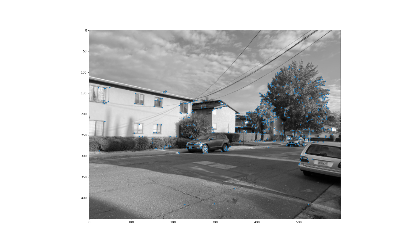
Part B1: Harris Interest Point Detector
In this part of the project, I used the given harris.py file to find Harris corners. Harris corners are excellent features to use as correspondences. Corners are unique since they tend to be surrounded by different values than themselves, so they're good to choose. Below is an image with the Harris corners overlaid. As you can see, there are a vast many of corners in the image!
|
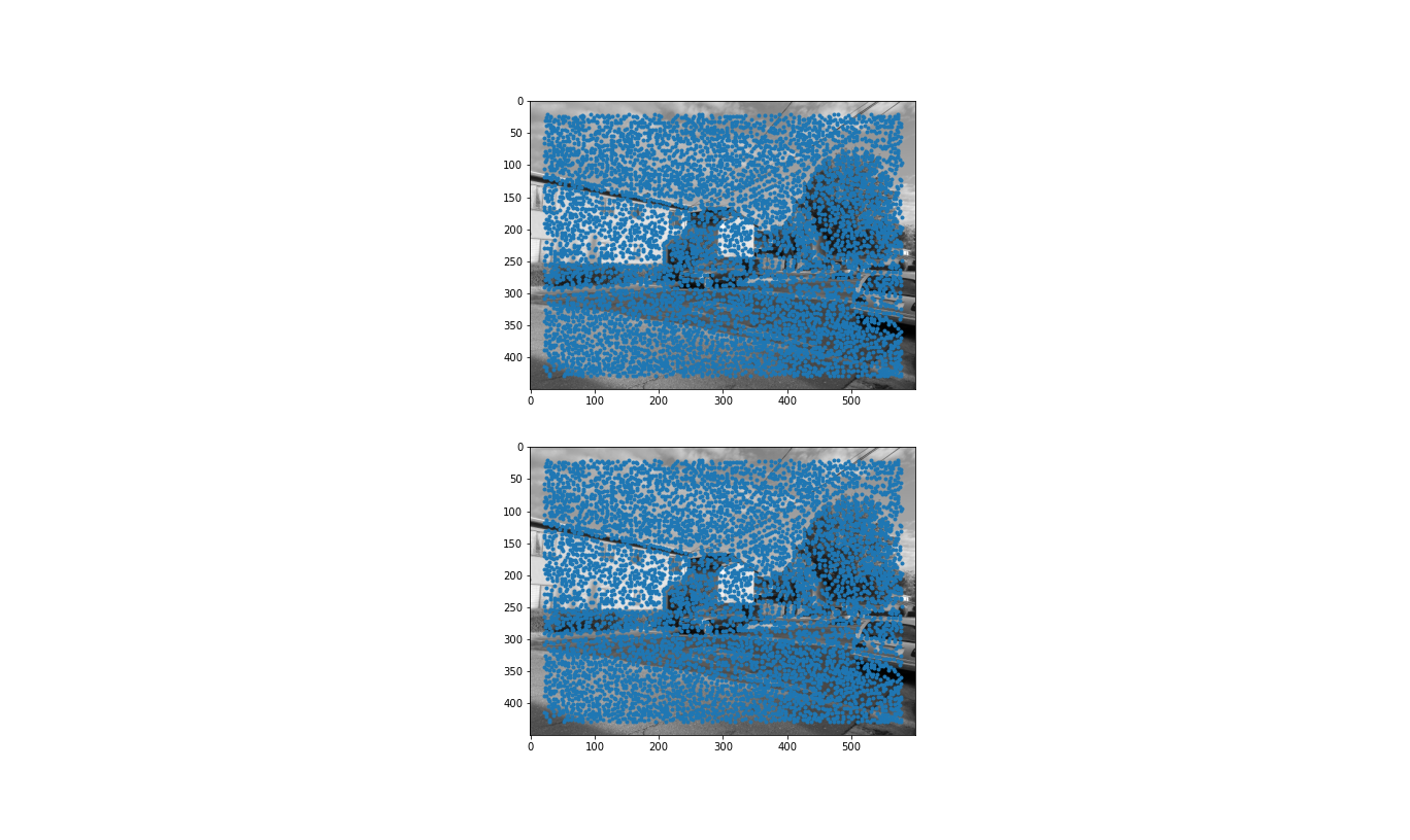
Part B2: Adaptive Non-Maximal Suppression (ANMS)
|
|
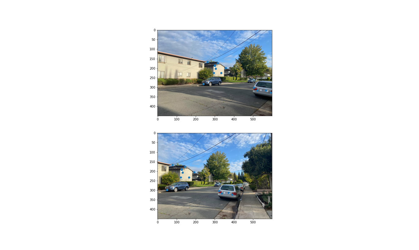
We care about getting a wide spread of easy-to-identify correspondences when we're generating our homographies. The Harris corner detector code gives us the strength of each Harris corner, given by det(H)/trace(H) of the Harris matrix at each pixel. We want strong corners, so naively, we could choose the 500 corners with the largest H values. However, we can see from Figure 12A that these corners tend to be clustered around areas where there are strong edges. In this example, the corners are along the tree, where it makes sense you'd see many corners (eg: branches, leaves). This strong clustering wouldn't be good to use to compute our homography, as it would heavily bias alignment in that region and ignore alignments elsewhere in the image.
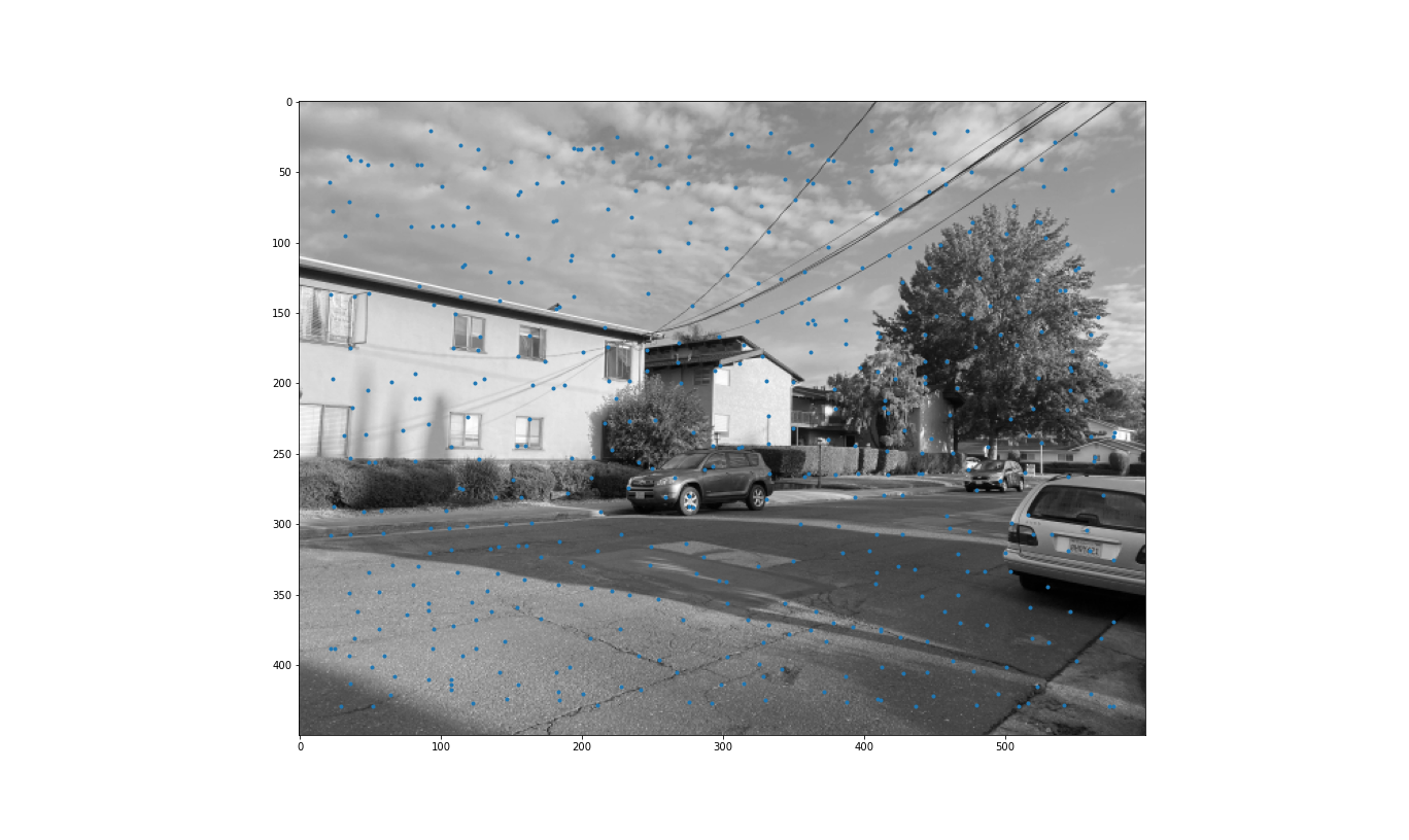
As such, we want to get strong corners that are spread throughout the image. To do this, we implement adaptive non-maximal suppression explained in "Multi-Image Matching using Multi-Scale Oriented Patches" by Brown et al. To do this, we find, for each Harris corner, the minimum suppression radius, which is a measure of how much stronger the corner is compared to nearby ones. the equation for this is shown below.

|
We care about the points with the largest values of r_i, which is to say they are stronger than the points in that radius of r_i. In our case, we choose 500 of the largest r_i's and use their corresponding Harris corners. The result is shown in Figure 12B.
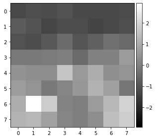
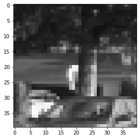
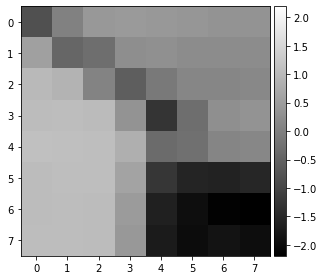
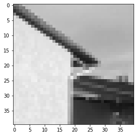
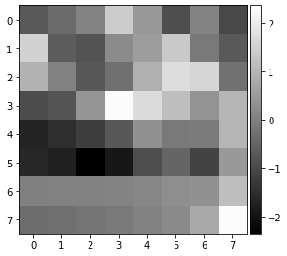
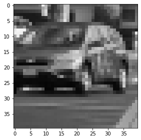
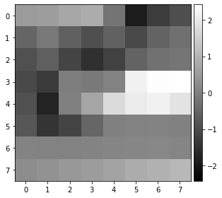
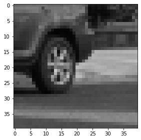
Part B3: Feature Descriptor Extraction
In this section, we extract 8x8 patches. For simplicity's sake, we do not rotate, and instead axis-align. For each of the selected interest points from B2, we extract the 40x40 patch centered at the interest point. We then down sample this patch until it is 8x8. This becomes the descriptor for this section. We also make sure to normalize the patch by subtracting the mean and dividing by the standard deviation so the mean is 0 and the standard deviation is 1.
A few examples are shown below, shown next to the original source patch to verify correctness.
|
|
|
|
|
|
|
|
The rest of Part B
Tragically, I did not get to complete the rest of this project due to a massive depressive episode :( I enjoyed what I did get accomplished in the project, so thanks for setting up this groundwork! That said, I hope to see my automated stitching to be more effective than my hand-stitching.
What have you learned?
Though maybe somewhat basic, I am still astonished that the pencil of rays allows us to get so much information through homographies. It makes sense that the data is present in the image, but it still is so astounding to me that you can "hide" images and extract them later through homographies.
I also learned how important keeping the center of projection still is. I didn't realize that it would have such a profound impact on my mosaics. Perhaps this is an indicator that I should invest in a tripod...
I'm also a big fan of Lowe's rule--or as Professor Efros likes to call it, Russian granny trick. It's amazing to me how such a simple idea can be so powerful.