Overview

In part a of Project 4, we implemented mosaicing of images of a common scene. In order to do this, we establish keypoint correspondeces between images, and then solve for the homography, or homogeneous transform, in order to warp pixels from one image to another image. In order to solve the homography, we place the keypoint correspondences in a matrix, where every 2 rows corresponds to a keypoint pair. Our data matrix, P, has the dimensions (n*2)x9.

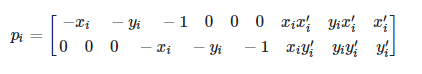
We can then solve for the homography vector H of dimensions 9x1 by solving for the null space of P (since we want the equation PH=0 to hold) and reshape it into our 3x3 homography matrix. We then perform mosaicing by morphing all images to a common plane Once we have these homographies, mosaicing involves several steps:

1. Forward warping the corners of each image to the common plane to find the bounding polygon from which to interpolate from
2. Inverse warping from inside the bounding box on the common plane to retrieve pixel intensities from the original images
3. Blending to reduce the harshness of borders separating mosaiced images

Improvements (Bells and Whistles)

Keypoint Refinement

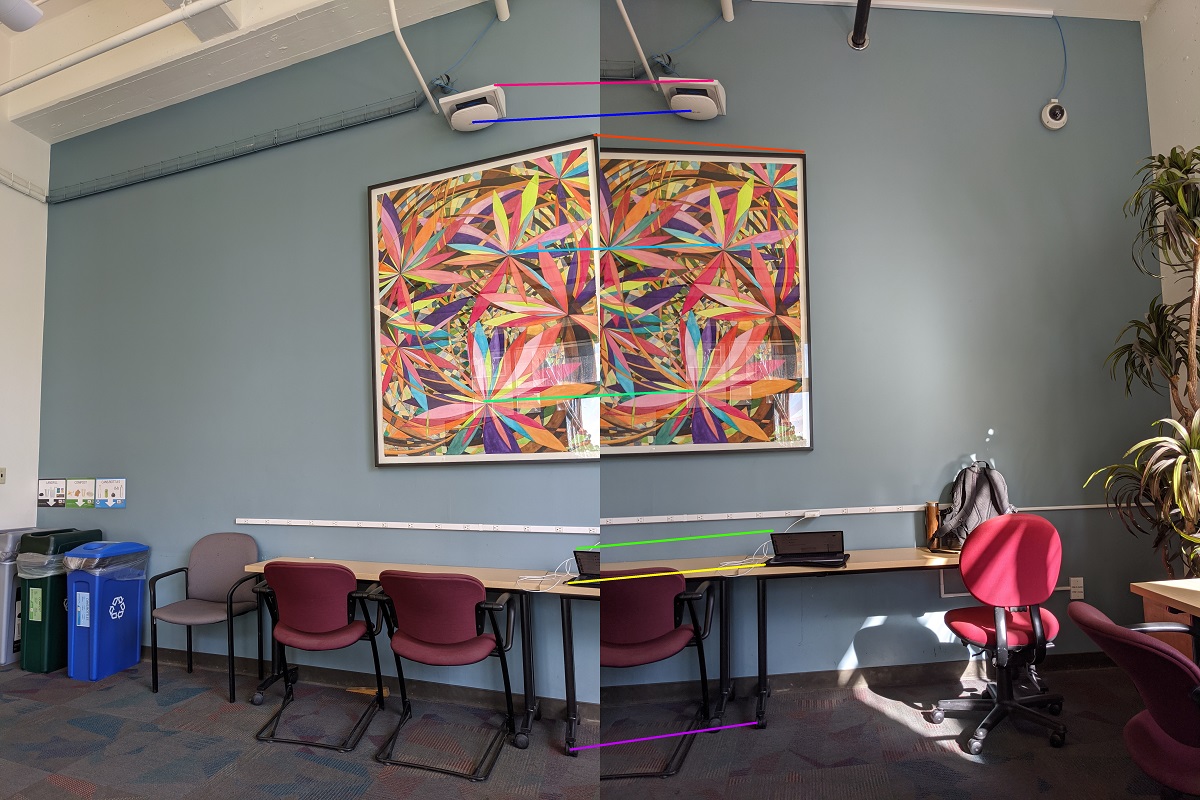
The process underlying all the homography calculation is the keypoint selection and correspondence. Having keypoints that are slightly off results in misaligned images. One method I used to combat this was refinement of the keypoints after manual selection. I did this using a process inspired by keypoint descriptors such as SIFT, doing a grid search of patches around the manually selected keypoint, computing a descriptor, and then selecting the keypoint with the descriptor most similar to the reference point. The descriptor is generated by extracting a patch around the point, calculating the gradient magnitude and direction at each pixel in the patch, binning the pixels based on gradient direction, and then summing up the magnitudes in each bin. I also introduce orientation invariance by aligning each patch such that the average gradient is always pointing in the same direction.

Image Mosaicing Results

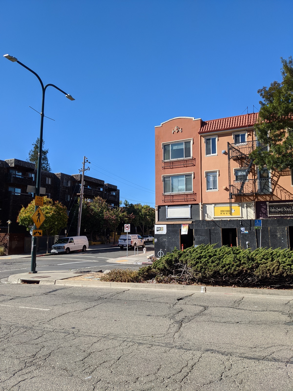
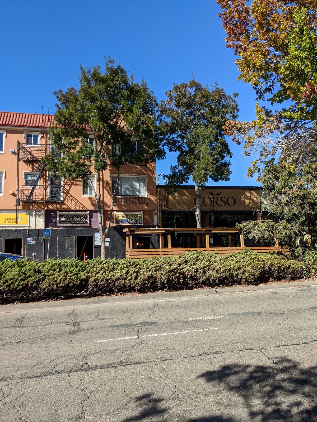
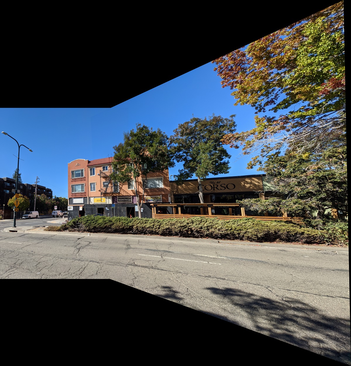
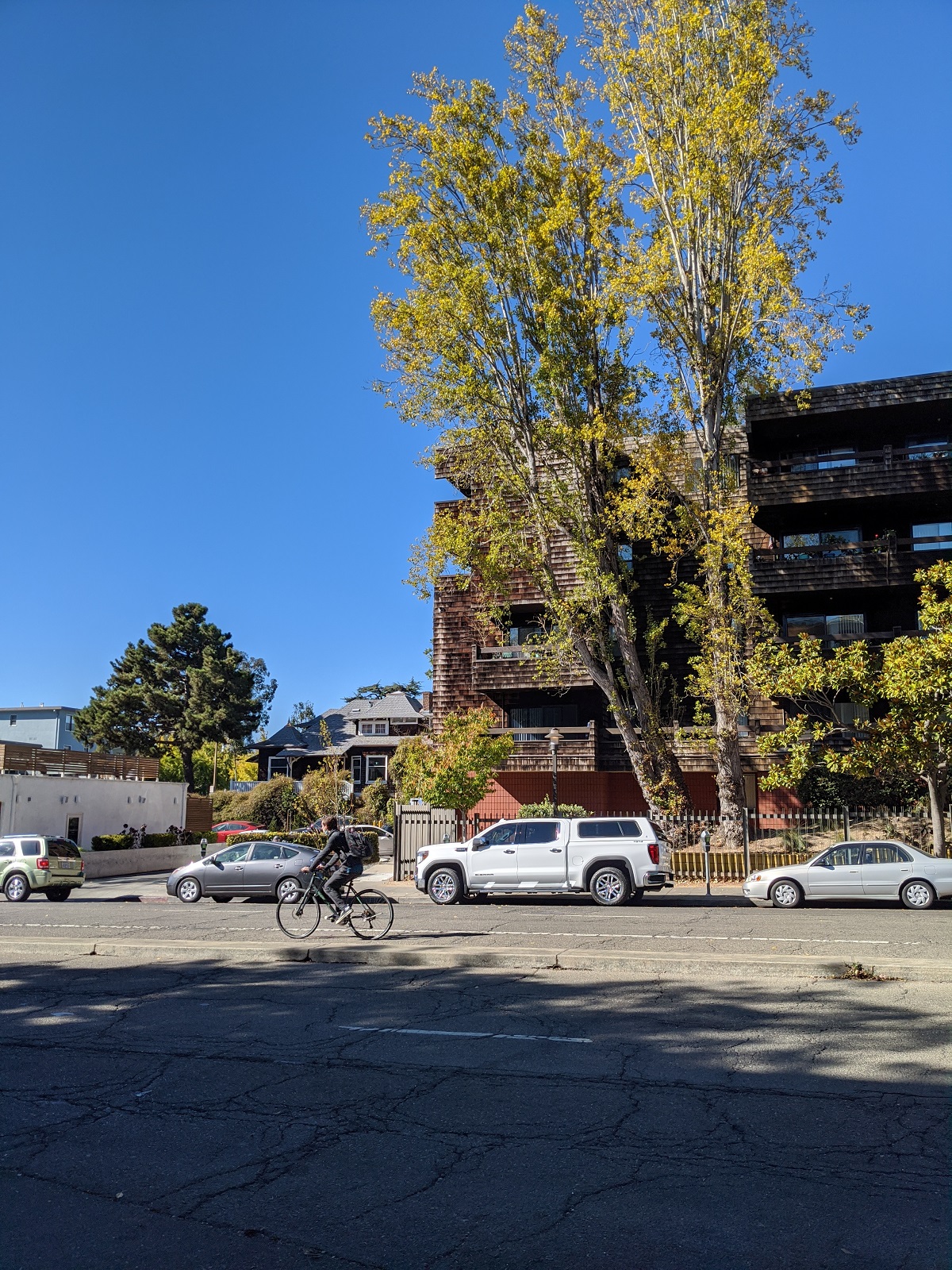
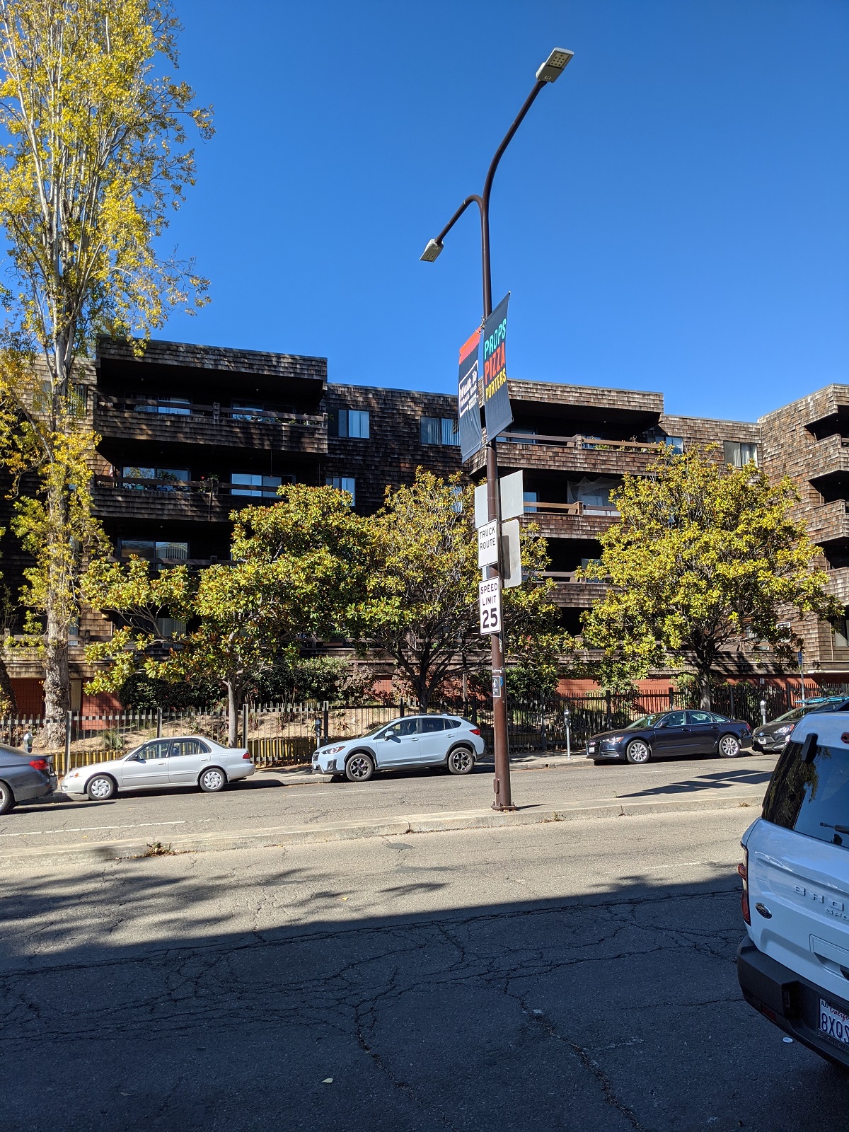
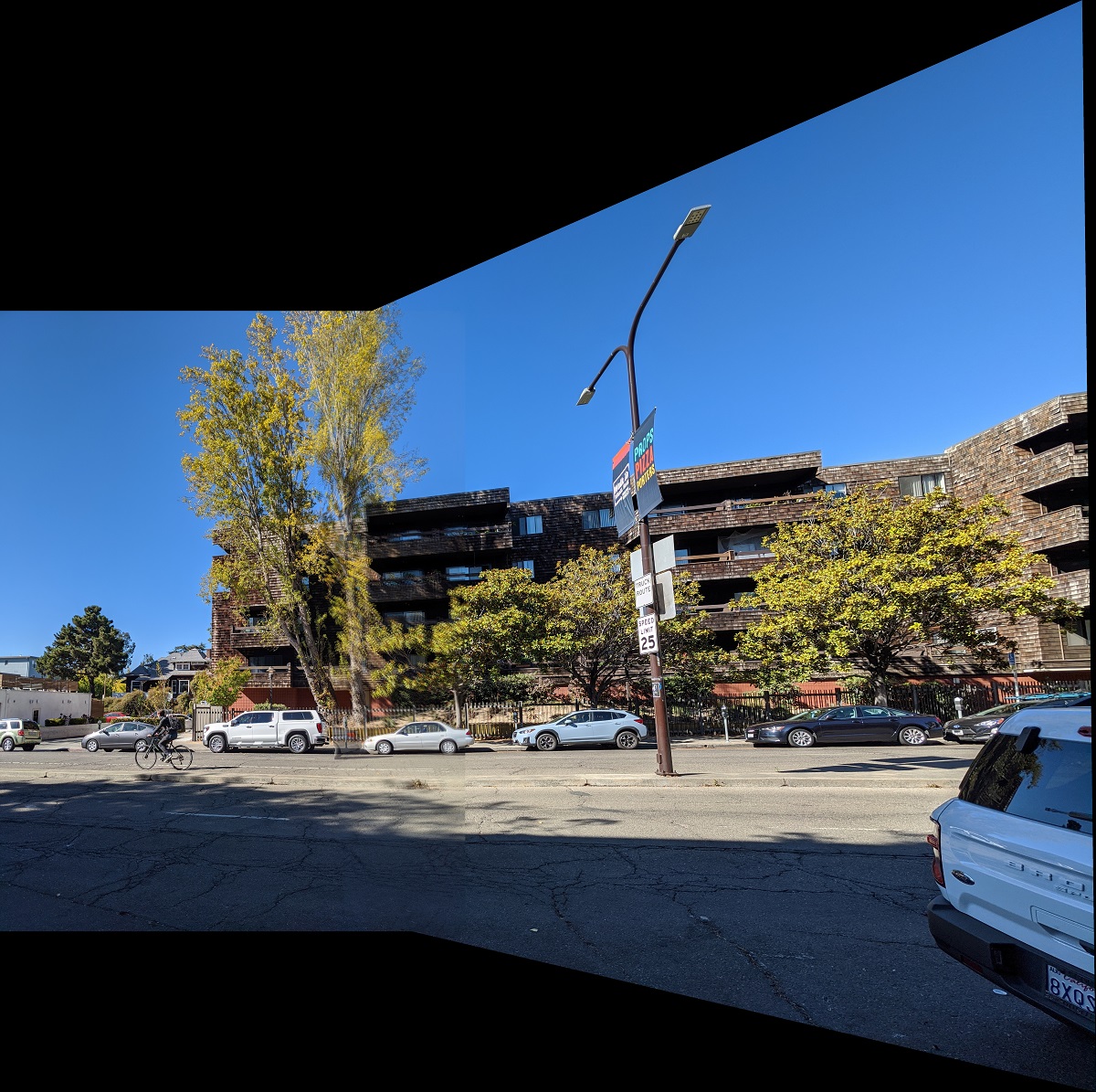
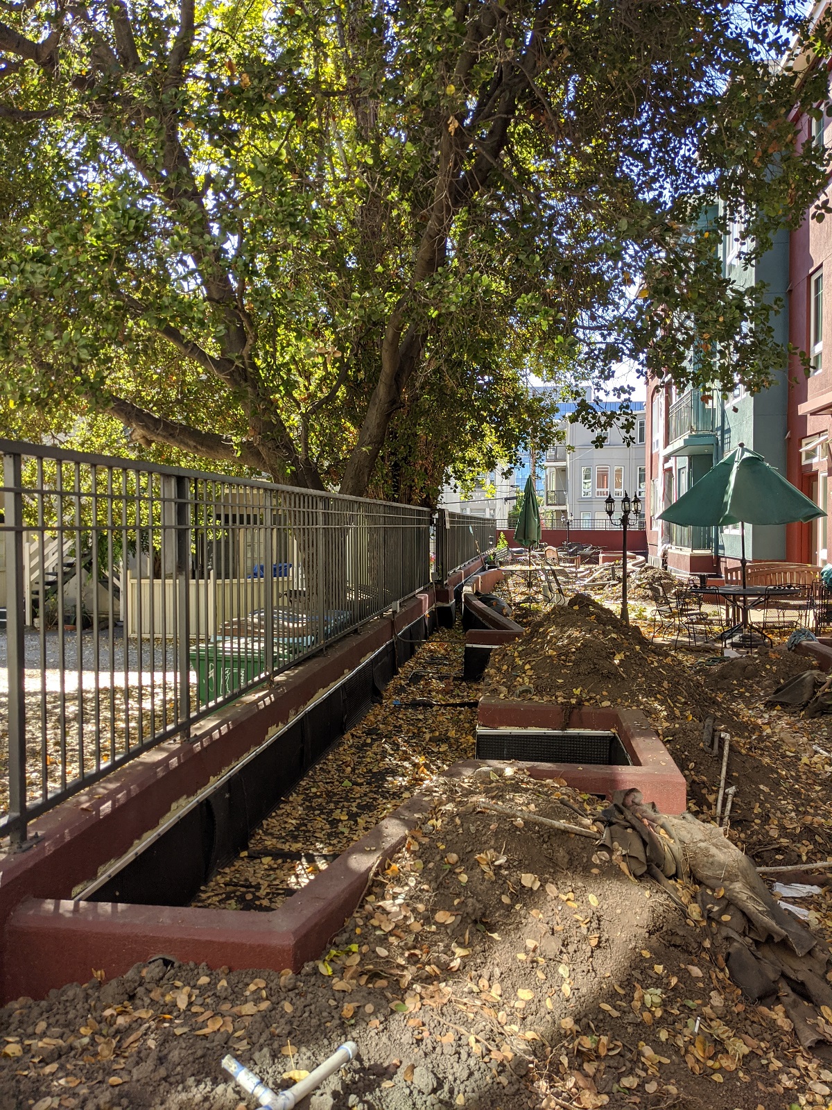
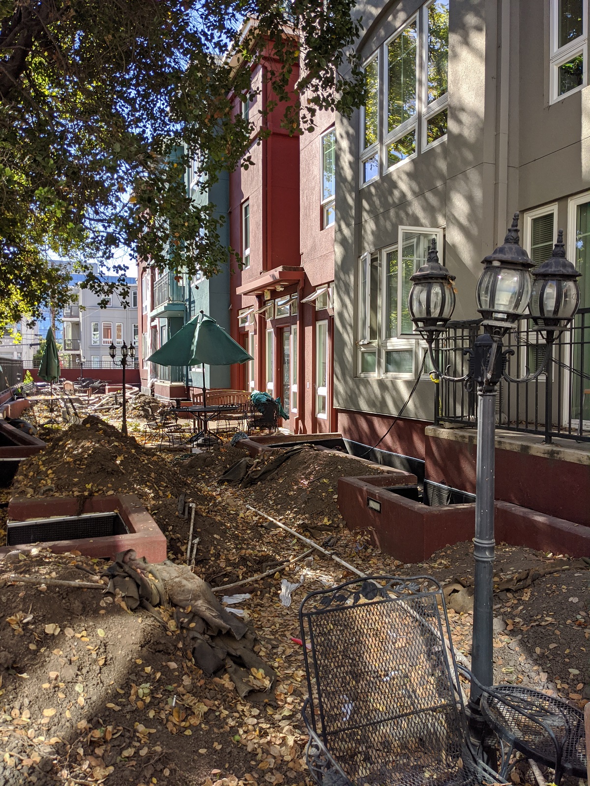
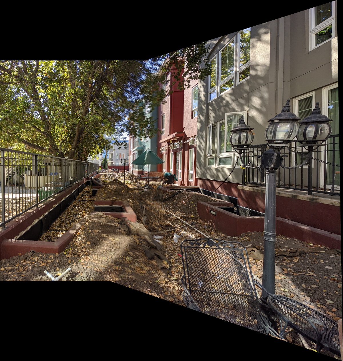
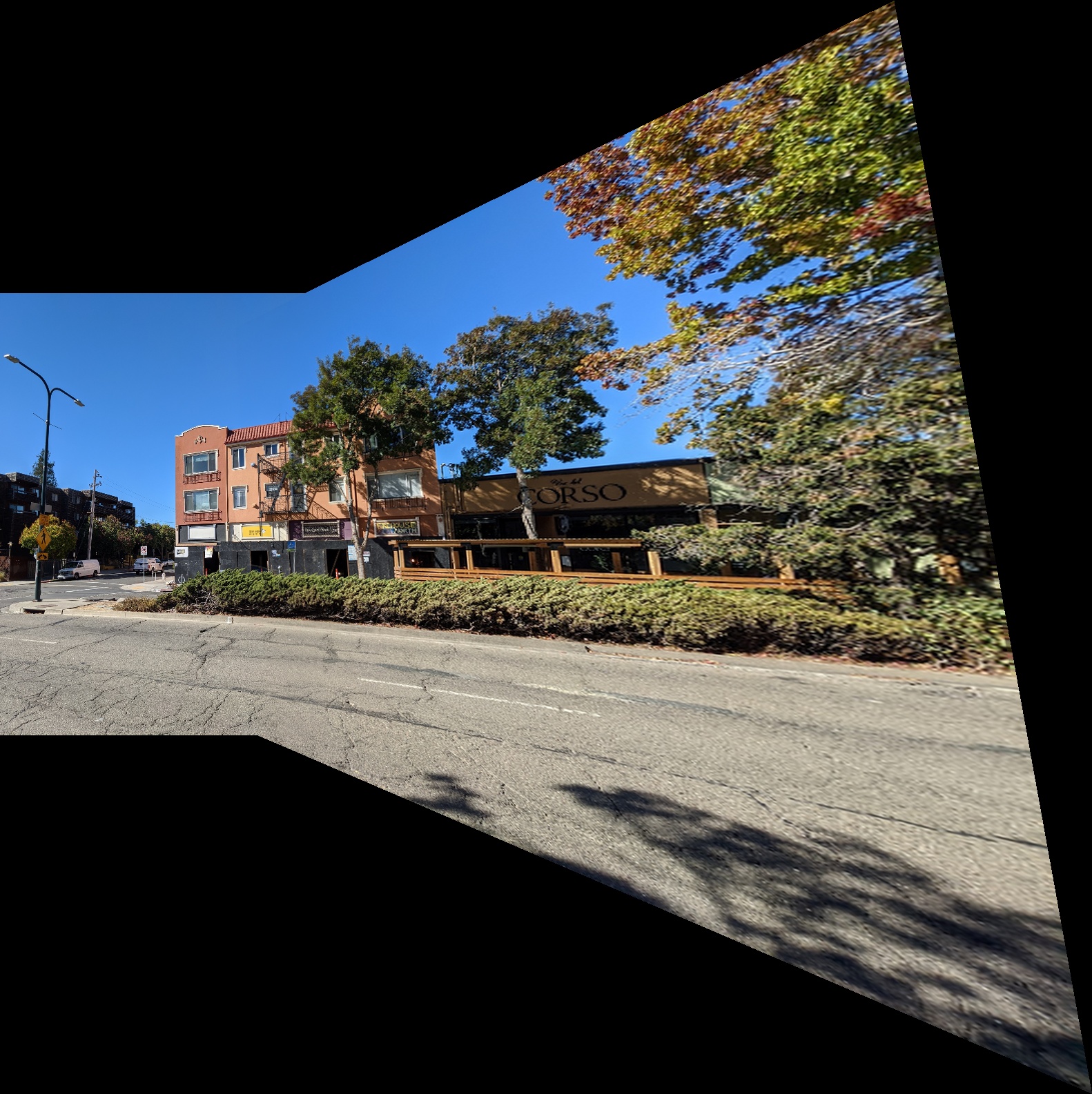
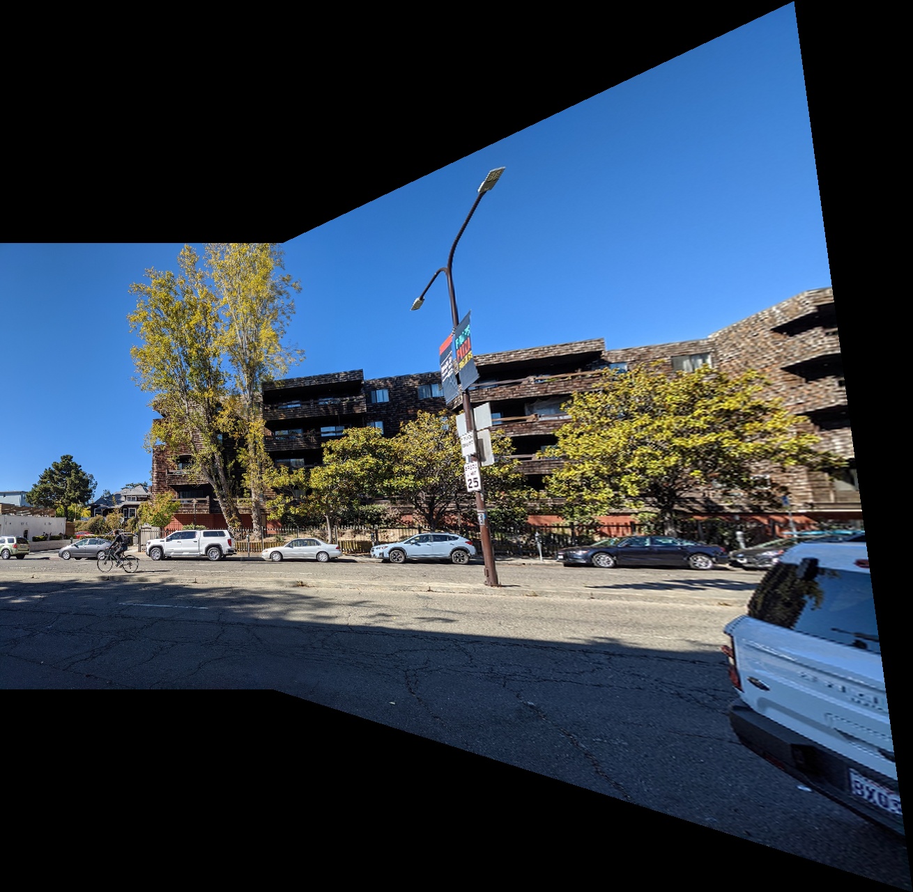
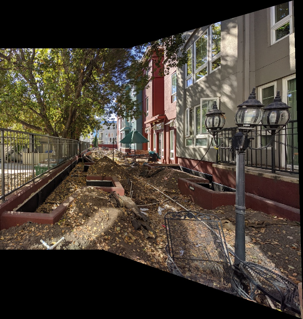
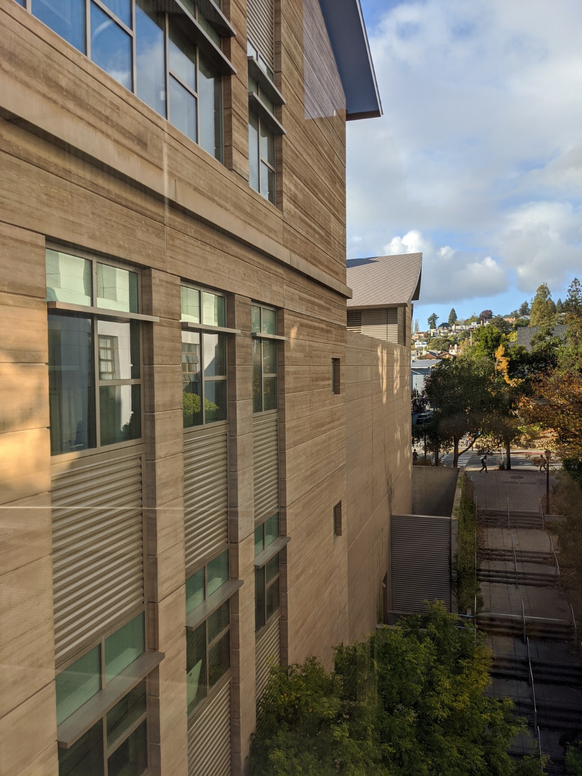
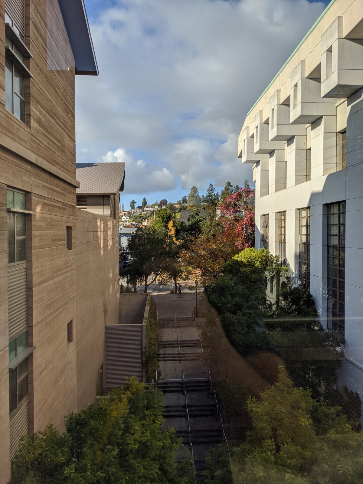
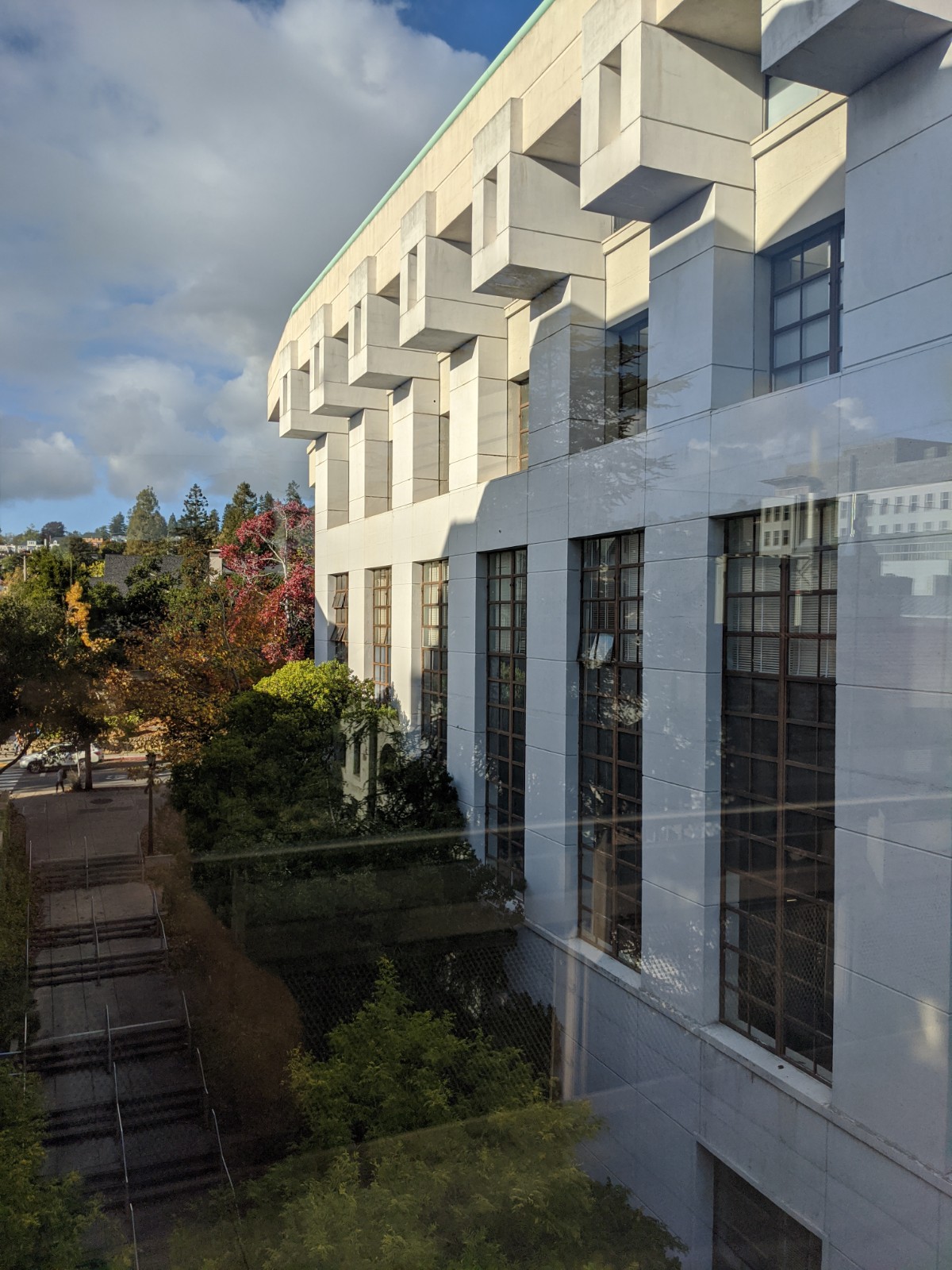
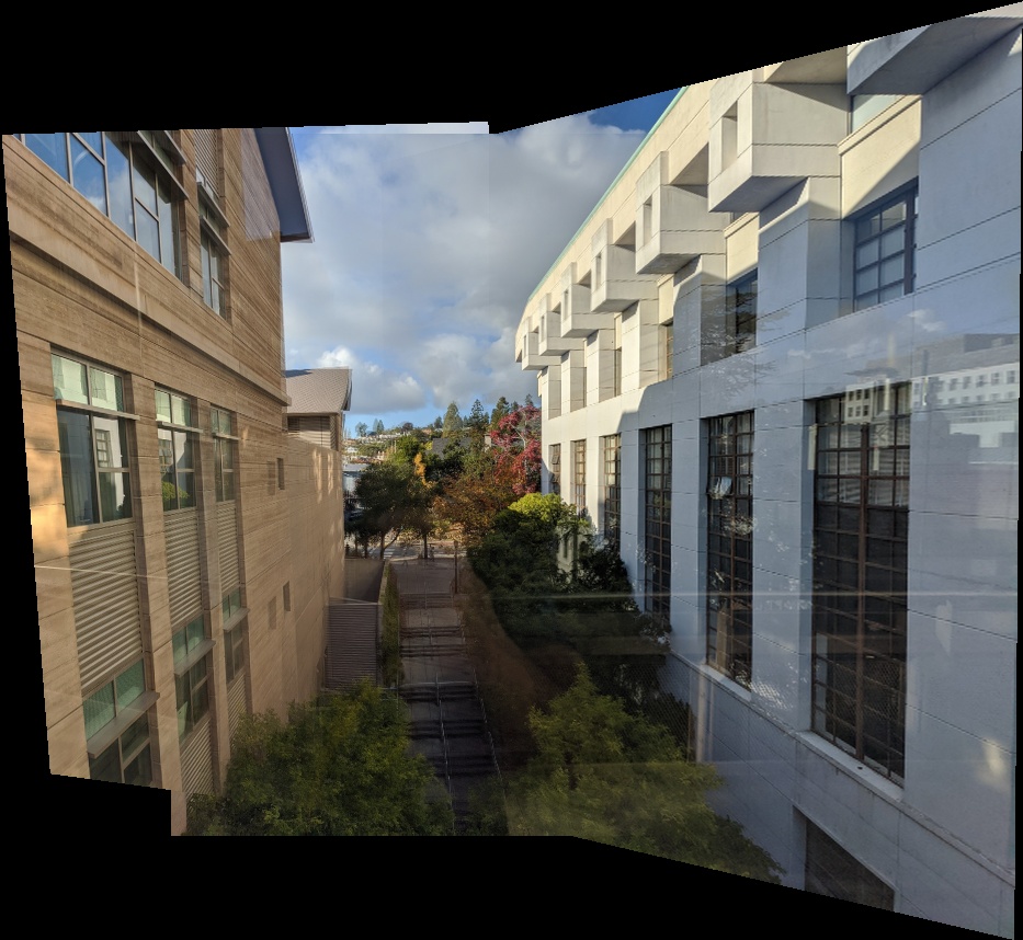
Below are results of performing image mosaicing.

Image A	Image B	Image Mosaic

Plane Rectification

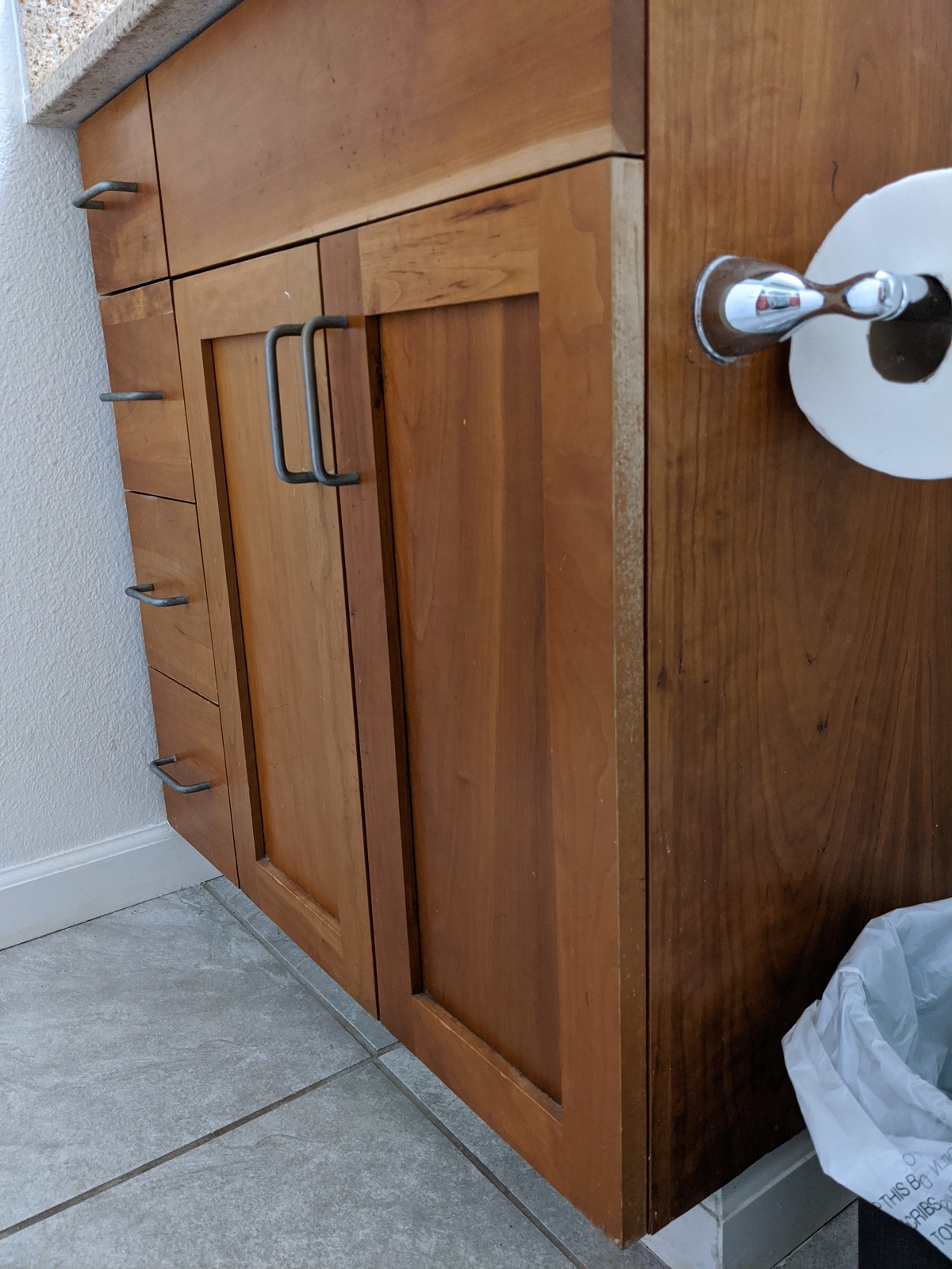
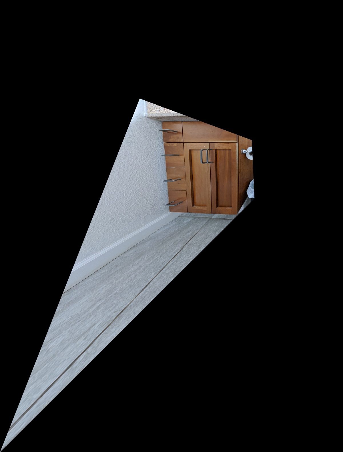
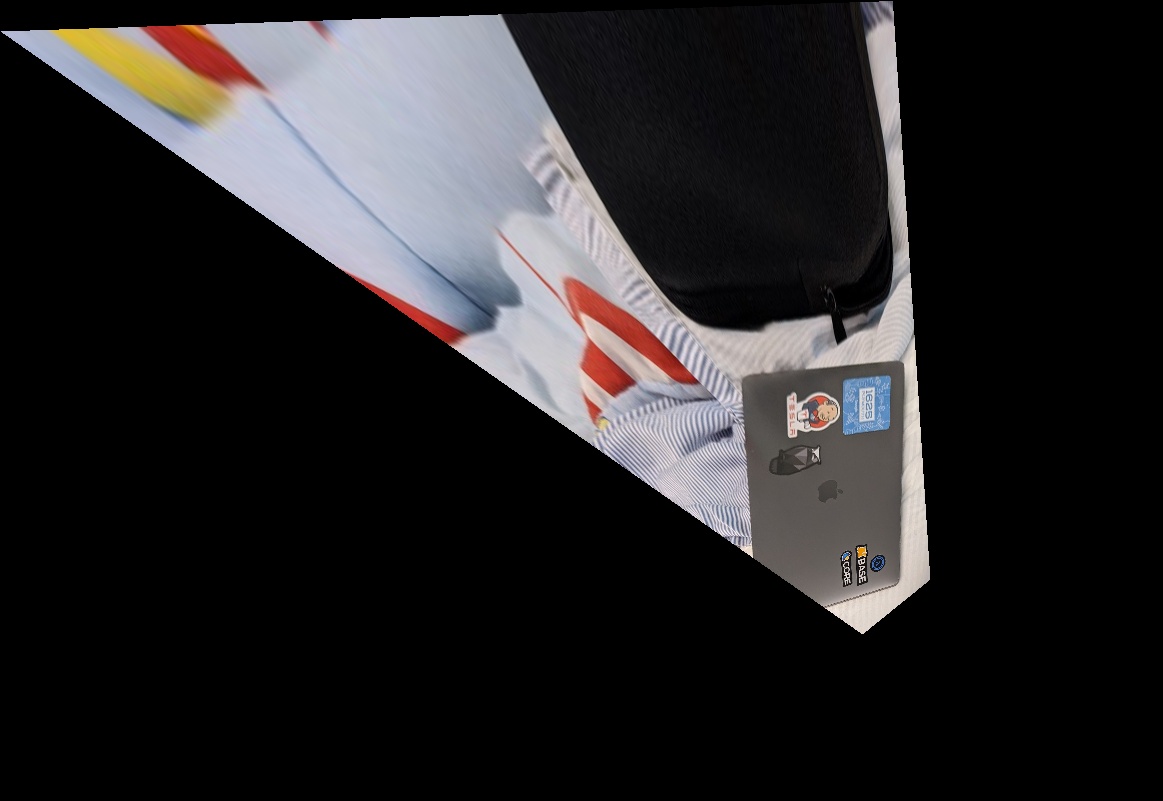
One last thing we implemented was plane rectification, both to sanity check our warp as well as develop some interesting results. Below are a couple of my rectification results. The first result really displays the shortcomings of our homography approach. It requires a planar assumption, and when the planar assumption is violated, the warp becomes very odd.

Original Image	Rectified Image

What I learned

I think the thing that I've learned the most is a newfound respect for panoramas in cameras. It seems very difficult to properly blend the images together, and its very difficult to algorithmically determine if there are errors in our mosaic. I also experienced the difficulty of working with very large images and the restriction my computer's memory imposes.

Overview

In part b of Project 4, we left the realm of manually selecting and refining keypoint correspondences between images, and instead used automated techniques to detect keypoints (harris corners), describe them (MOPS descriptor), and match them using nearest neighbors with some modifications. We also learn to compute homographies from noisy correspondences using RANSAC.

Detecting Corners

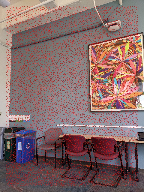
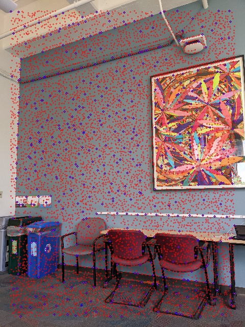
The first thing we implemented/used was a feature detector. We want to select a subset of all the pixels in the image to actually perform the downstream tasks on. This is for several reasons. First, we want to reduce the computational complexity of our problem. Secondly, matching some pixels is not possible, for instancer, if they are part of some featureless plane. We select keypoints from our image using a Harris Corner Detector as described in lecture. It is a simple technique that detects corners based on the intuition that the second derivative of the Gaussian window around each point will be a local maxima. Below is a visualization of Harris Corners detected on the image. We see that there are many corners detected, many of which don't seem to correspond to an actual corner. These are the result of imperceptible but very high frequency changes in the image due to noise.

Adaptive Non-Maximal Suppression

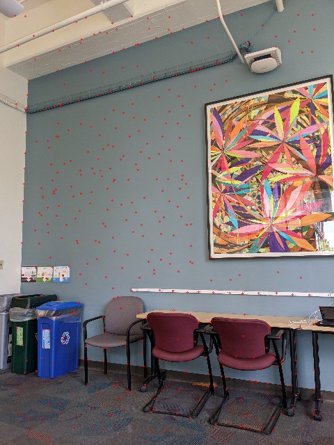
To address the issues laid out in the previous section where many spurious corners were detected in the image, we first apply adaptive non-maximal suppression as described by the paper "Multi-Image Matching using Multi-Scale Oriented Patches". This process involves suppressing non-maximum features such that the resulting selected keypoints are the maximum in their own uniformly distributed image area. Below are visualized the results of suppression.

Feature Descriptor

After extracting the most salient features in the image, we need a way to describe them such that we can perform our downstream task of matching keypoints between different images. We implmenet descriptors using a process similar to that which is described in "Multi-Image Matching using Multi-Scale Oriented Patches". We sample an 8x8 region around the keypoint, on a 5 times downsampled version of the image. We basically are extracting a low resolution 40x40 region around the keypoint to generate our descriptor. We then bias and gain normalize the descriptors. Below are a few examples of feature descriptors.

Matching

After performing description, we perform matching on sets of keypoints and descriptors from two different images. We begin the matching process by finding the nearest neighbor in the opposing set of keypoints for each keypoint from either image. We then perform pruning to remove incorrect matches. The first pruning step involves enforcing cyclic consistency. If a keypoint in Image A, K_a, has a nearest neighbor in Image B, K_b, then this correspondence is pruned if the nearest image in Image A for K_b is not K_a. The second pruning step involves a ratio test between the first and second nearest neighbor for keypoints in Image A. Given a keypoint K_a in Image A, let the first nearest neighbor in Image B be K_1 and the second nearest neighbor in Image B be K_2. The correspondence (K_a, K_1) is pruned if dist(K_a, K_1) / dist(K_a, K_2) is not below a certain threshold. This intuitively only allows correspondences that are deemed reliable.

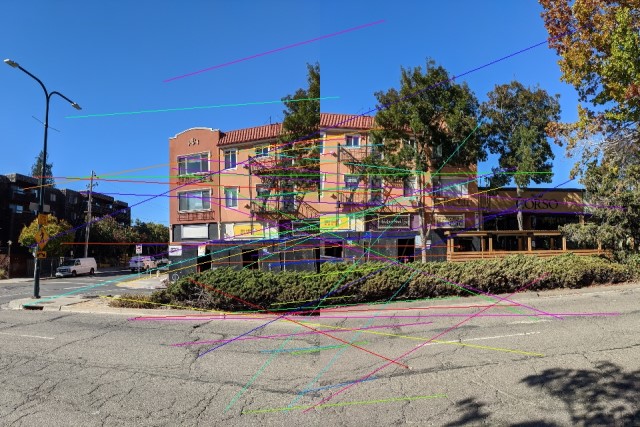
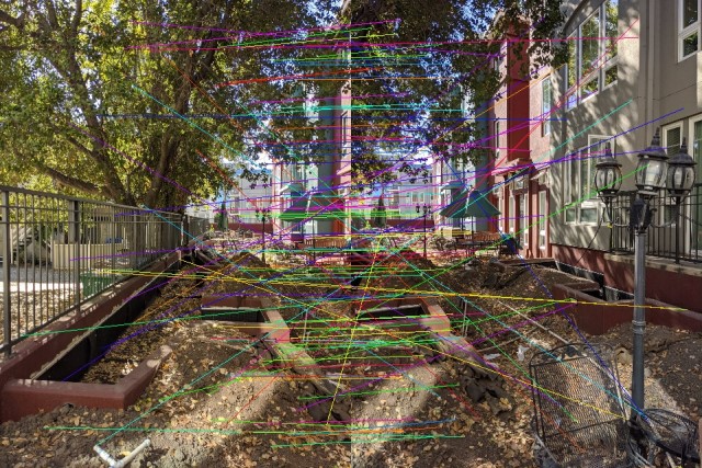
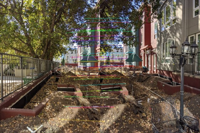
Below are visualizations of the correspondneces between 2 images with the two pruning techniques already applied: We see that there are still many incorrect correspondences.

Homography Calculation using RANSAC

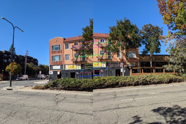
In part a of Project 4, we used a direct linear transform to calculate the homography between the 2 images. This technique would lead to failures in our new scheme due to the existence and proliferation of outliers. Therefore, we must use an algorithm called RANSAC in order to calculate a homography robust to these outliers. RANSAC uses noisy data to estimate a model that fits a non-noisy subset of the data. It does this by iteratively estimating a model, then segmenting the data into an inlier set and an outlier set. It uses the inlier set to update the model, repeating until the inlier set grows to a certain threshold. We can see the effect of RANSAC below. On the same image pairs shown in the previous section, we see that RANSAC has extracted the inlier set corresponding to the true homography:

Results

We can compare results from part a and part b. One of the major benefits of using auto keypoint matching is the mitigation of slight misalignment errors. The overlapping regions in the mosaic between the input images doesn't have weird ghosting effects since they are truly properly aligned.

Part A Result	Part B Result

And one last result from part b:

The Coolest Thing I Learned

I think the visualization of how effective RANSAC was at recovering an inlier set from a set of noisy data was really cool. Several times, I thought there was an issue with RANSAC not finding my correct correspondences. Each time, though, it turned out the issue was somewhere else in my pipeline, and RANSAC was performing just fine and there simply wasn't an inlier set to converge to.