

Part A: Image Warping and Mosaicing
Recover Homographies and Warping
Image Rectification
Blending Images into a Mosaic
Additional Examples
Reflection
Part B: Feature Matching for Auto-stitching
Harris Interest Point Detection
Adaptive Non-Maximal Suppression (ANMS)
Extracting Feature Descriptors
Matching Feature Descriptors
Computing a Homography with RANSAC
Warping and Blending
Additional Examples
Reflection
In order to perspective-warp one image to another, we need to compute the transformation matrix, which in this case is a homography. The homography is a 3x3 matrix with 8 degrees of freedom (the bottom right entry of H is a scaling factor and can be set to 1.)
Figures by Zadeh
To recover the homography, we need pairs of corresponding points from the two images. Four correspondences are needed to fully recover the homography matrix, though using more than four may produce more desirable results. With four, we can simply solve the following linear system of equations, Ah = b, where h is a vector containing the entries of H, and b is a vector containing the x and y coordinates of the destination image's correspondence points.

Figure by Zadeh
As was previously stated, it may be beneficial for us to use more than 4 correspondences because it may result in a more stable homography recovery. In this case, we will need to solve the over-determined system with least-squares, but the equation setup is similar to the one above.
Once we have the homography, we can warp the images. I decided to use inverse warping, which applies the inverse homography matrix to destination image pixels in order to sample source image pixels.
Rectification by Criminisi, Kemp, Zisserman
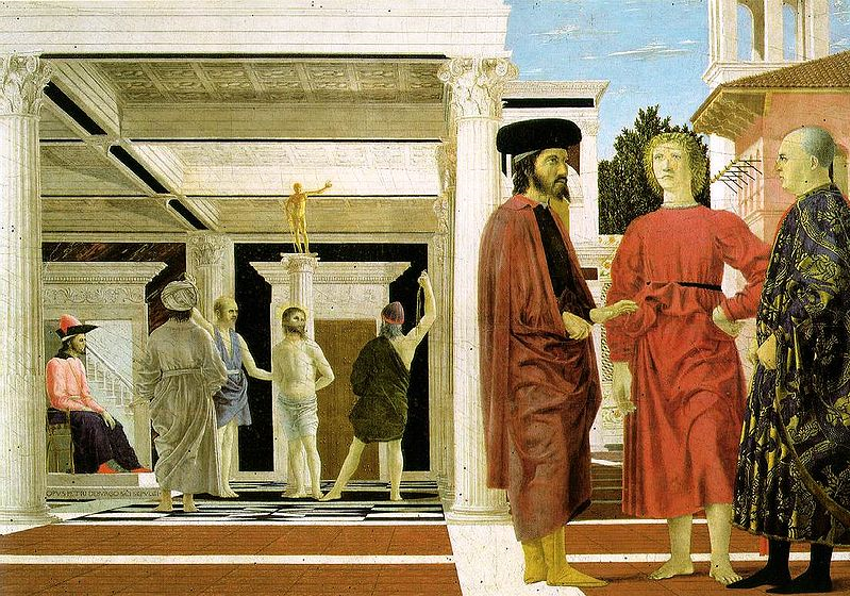
Suppose we would like to view the floor pattern in the painting, Flagellation of Christ by Piero della Francesca. Or perhaps, we would like to view a planar surface in a front-facing view. We can do exactly this through image rectification.
With a homography and a warp function, we can now "rectify" images that contain planar surfaces so that the planes are frontal-parallel.
This is done by warping the surface in the image to a rectangle.
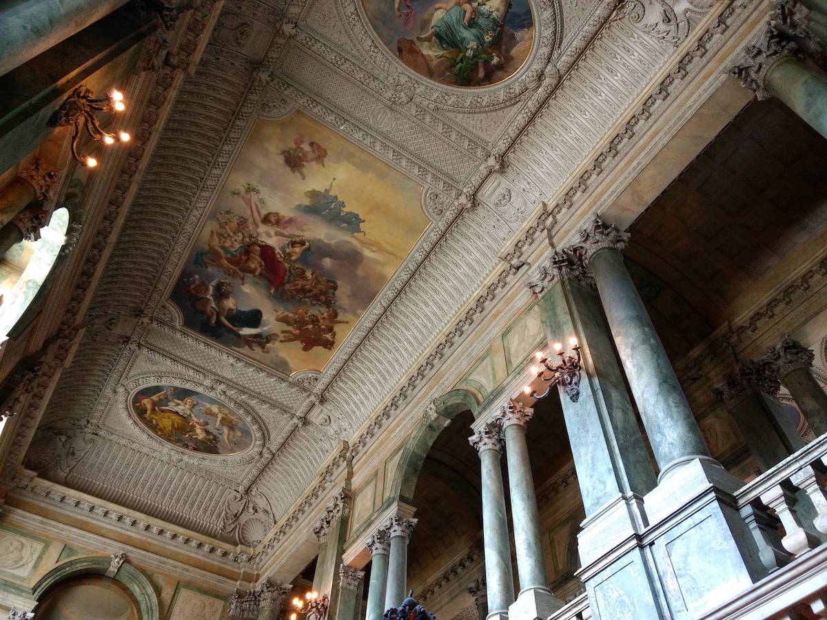
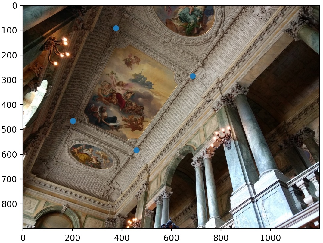
For example, below is a ceiling painting that has been rectified.
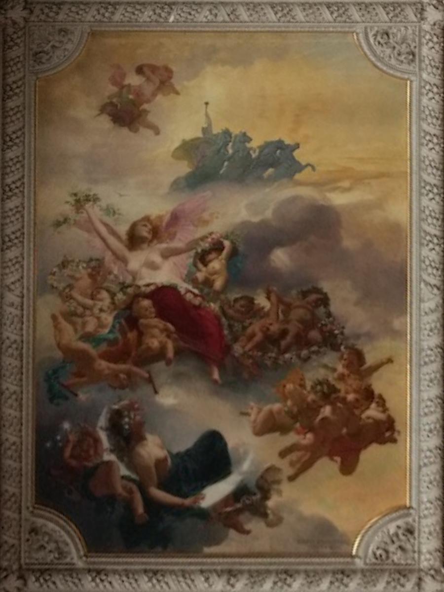
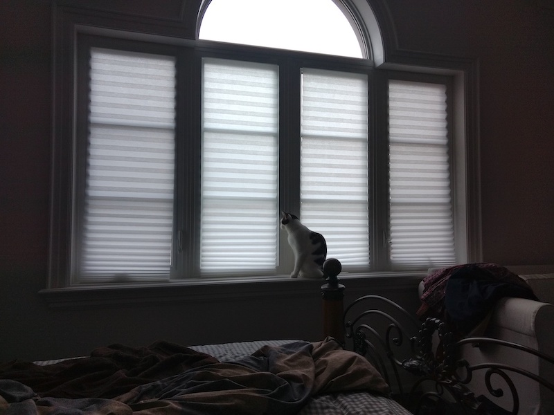
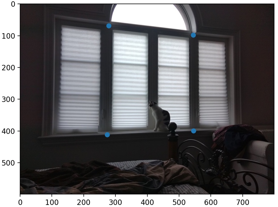
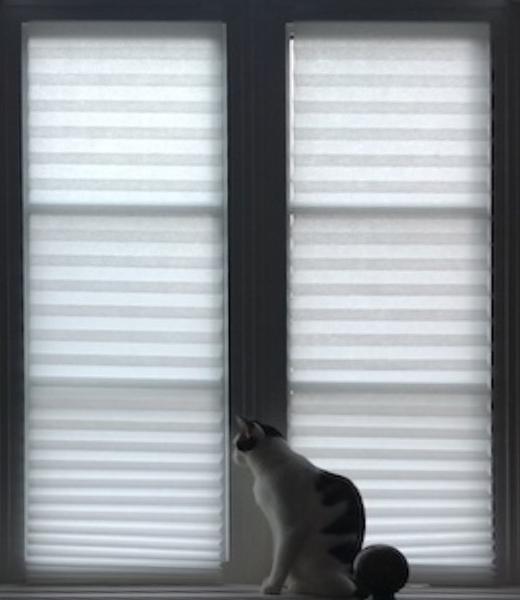
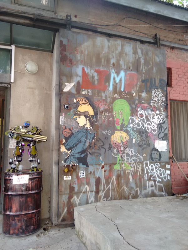
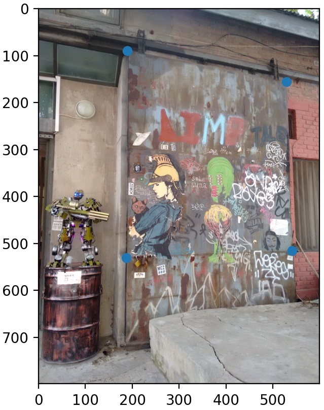
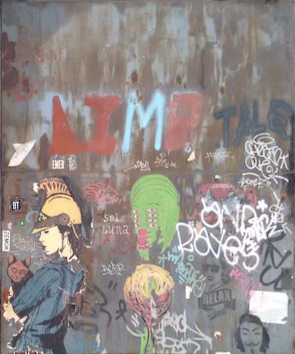
The same can be done with walls, windows, museum paintings, etc. Here are two more examples, one of a cat sitting in front of a window, and another of graffiti:
With homographies and warping, we can also blend images into a mosaic (aka a panorama.)
There are several things to consider when shooting the photos though:
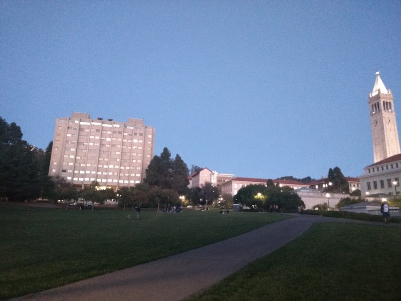
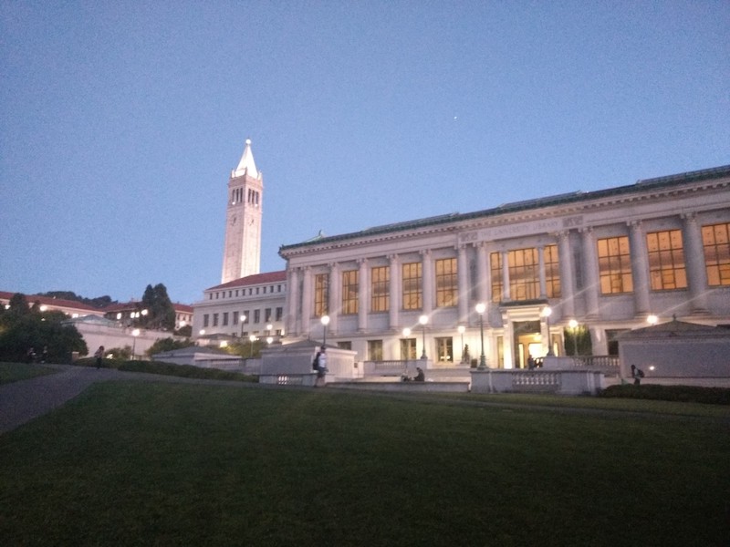
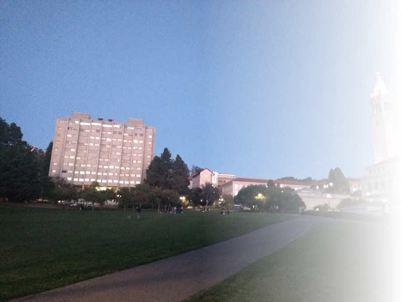
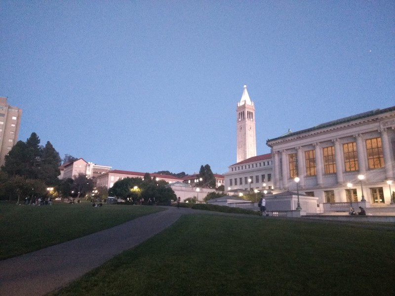
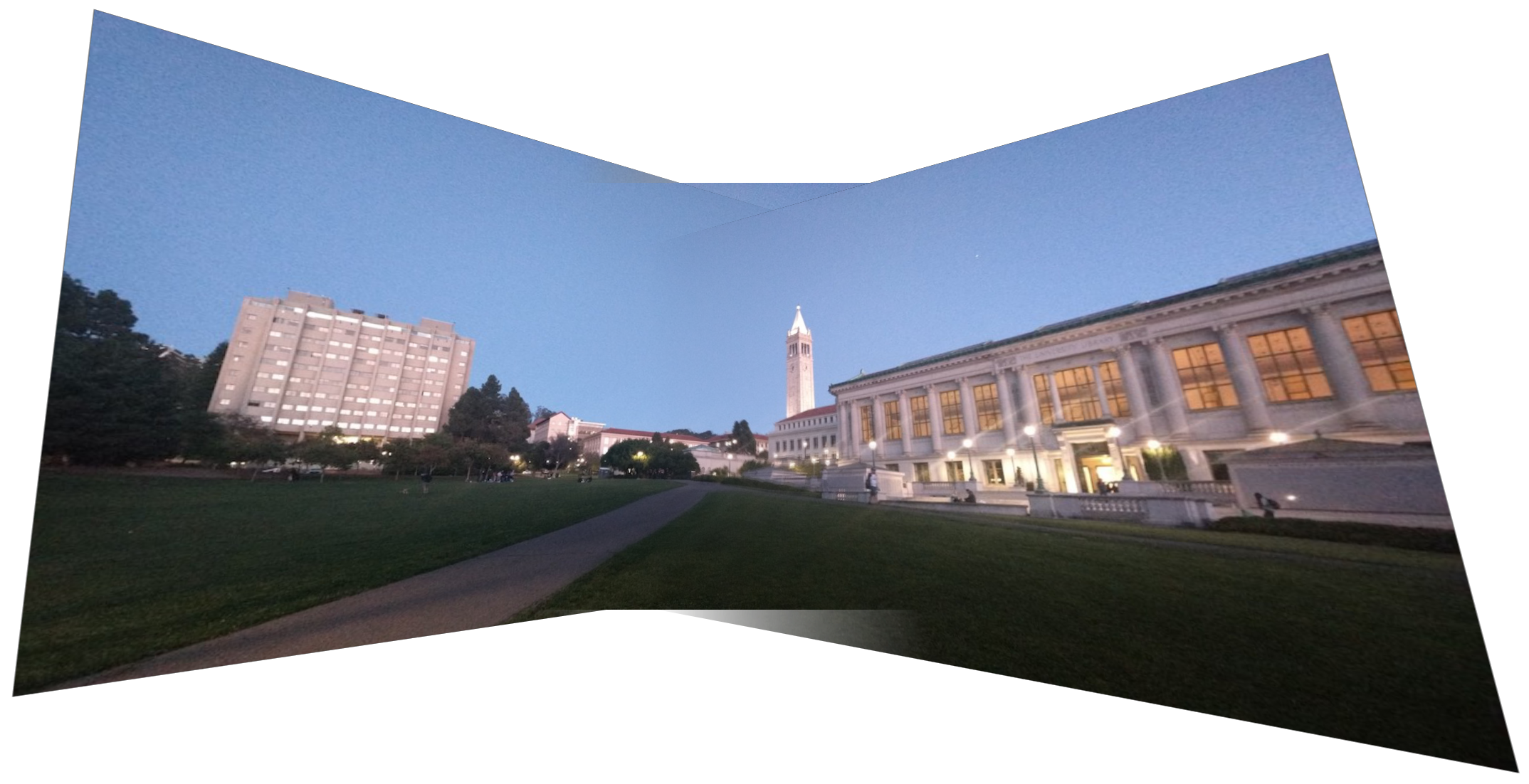
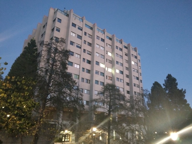
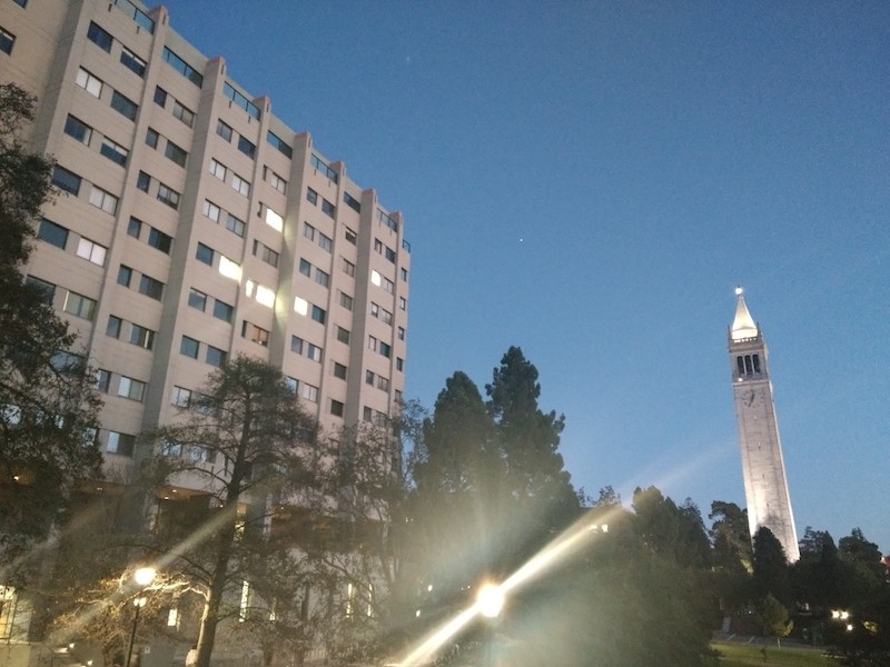
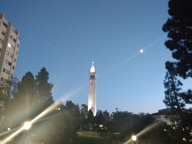
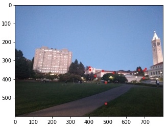
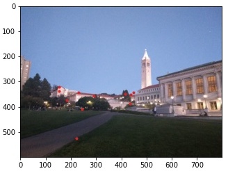
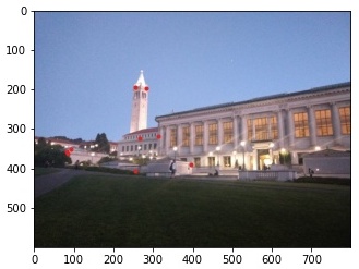
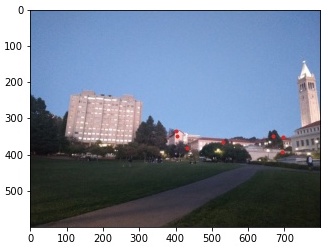
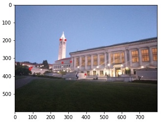
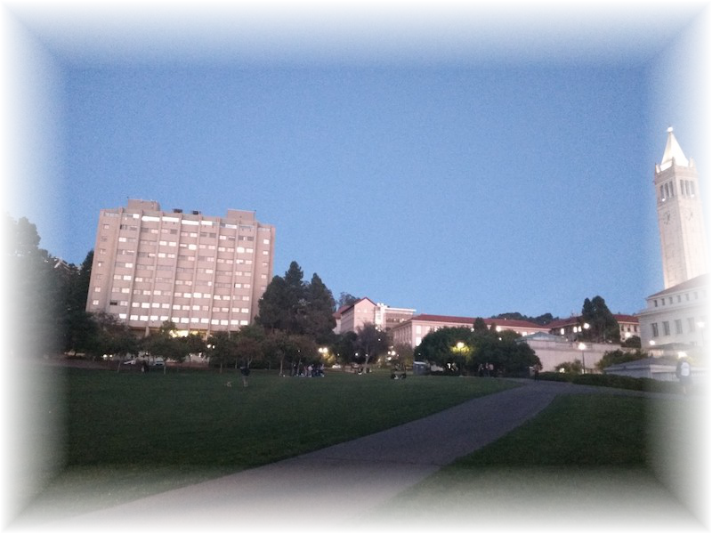
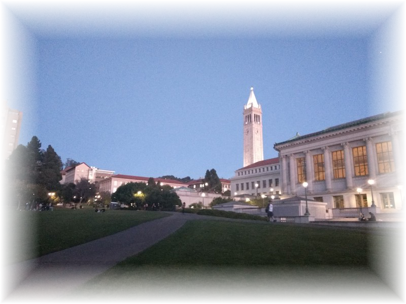
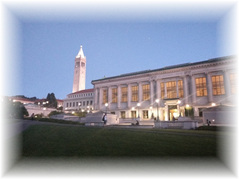
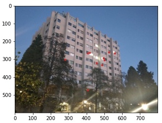
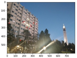
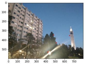
Here are three images I took of Memorial Glade:

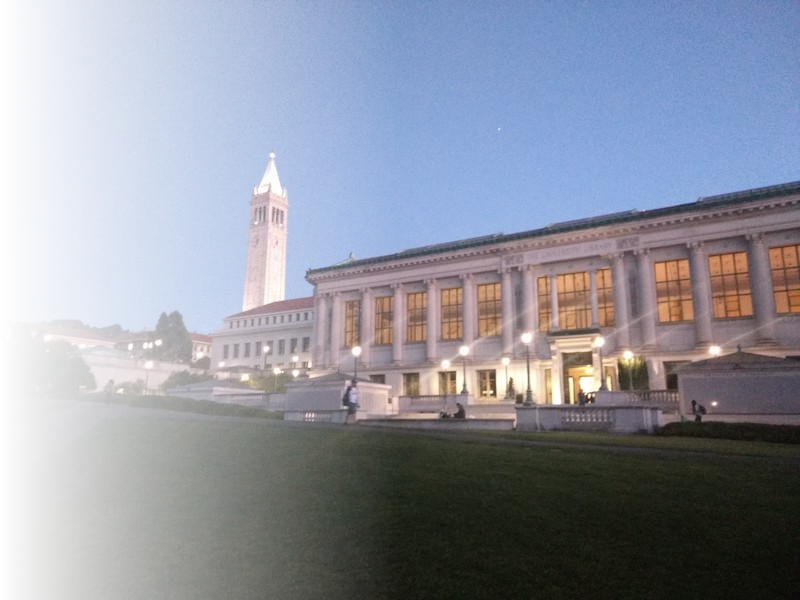
Before warping these photos, I added an alpha channel mask to each image so that the image is more transparent near certain borders that I specify. This will help prevent harsh edges when we blend the photos.
Now, we can define the correspondences and warp the images onto a large canvas.
Afterwards, we blend the warped images together with simple alpha blending.
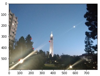
Below is the resulting Memorial Glade mosaic.
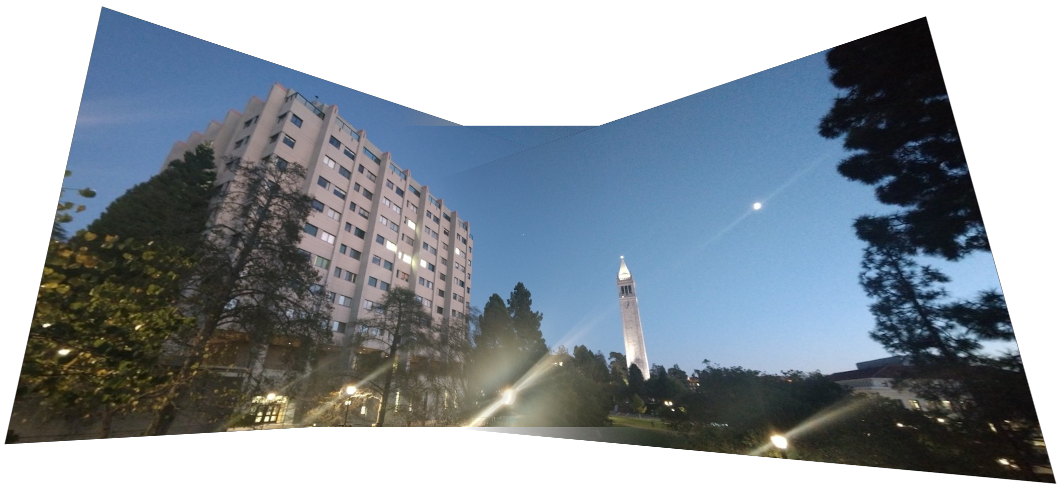
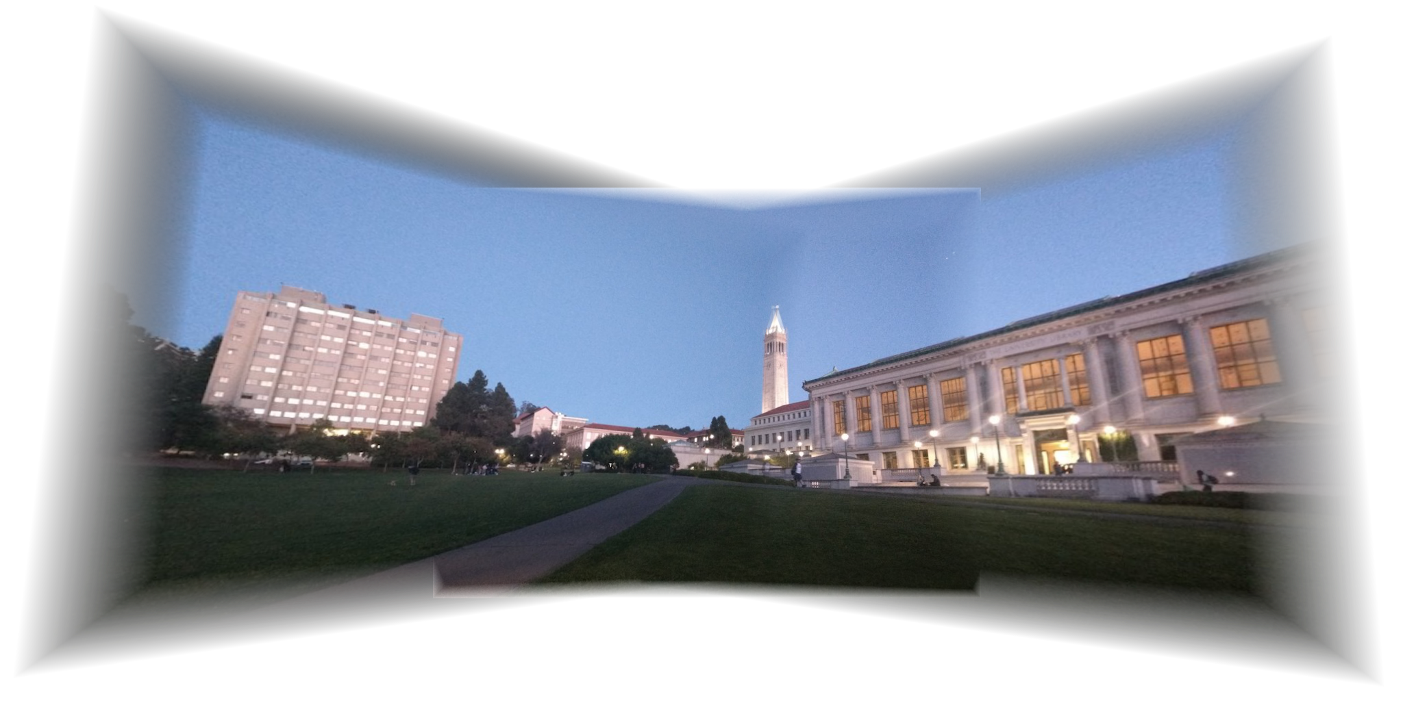
The same procedure can be applied to produce more mosaics!
Below are some more photos from campus and their mosaics:
I thought it was cool that surfaces in paintings, like floor patterns, that we normally would not be able to visualize, could be reconstructed using image rectification.
For more practical applications though, with image rectification, I can redeem all my poorly-taken museum photos...
As for image mosaicing, there are several areas I can improve on. In particular, the blending is not perfect, and this may be improved with a Laplacian stack.
Also, there is probably a better way of creating the alpha transparency masks for the original photos than the way I did so.
Overall, I learned a lot, and it was rewarding to see all the final images.
In Part A, we had to choose correspondence points by hand to compute the homographies. Now, we would like to automate this process. The following sections outline the procedure for doing so, which is based on the method in this Multi-Image Matching paper by Brown, Szeliski, Winder.
First, we need to detect the interest points.
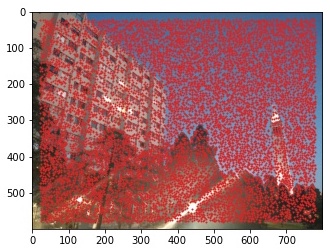
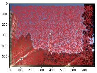
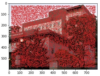
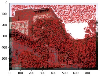
As previously stated, we don't want to manually select these points anymore, so here we will use Harris corners as the interest points.
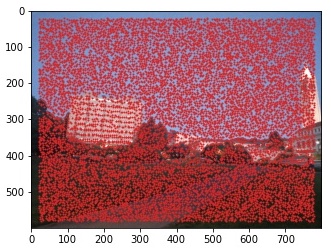
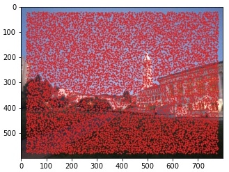
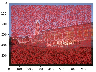
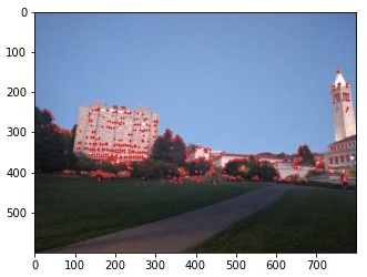
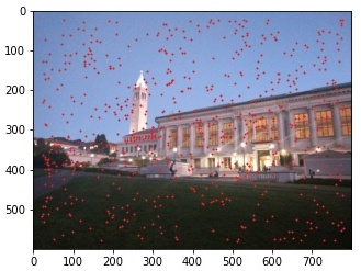
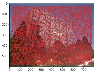
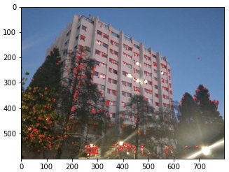
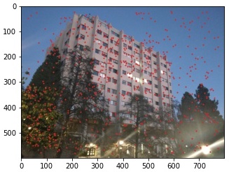
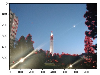
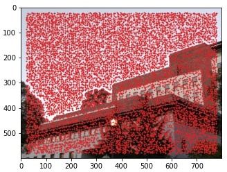
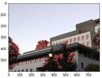
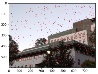
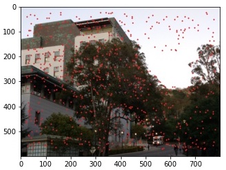
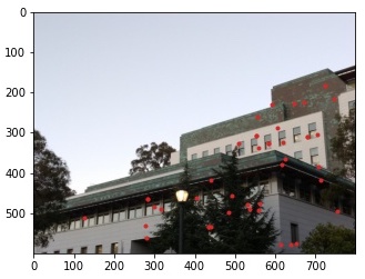
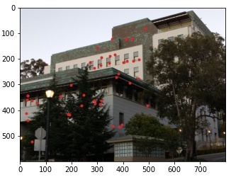
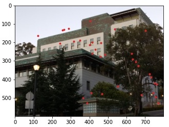
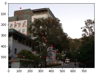
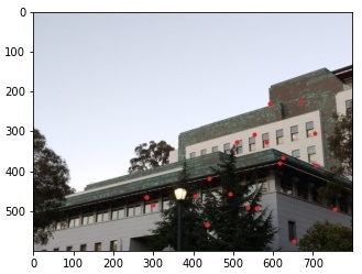
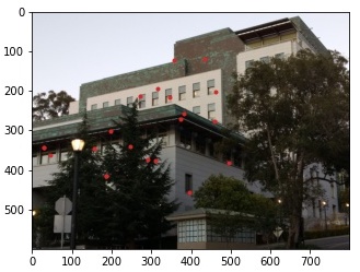
Below are the three images we want to mosaic and their Harris points.
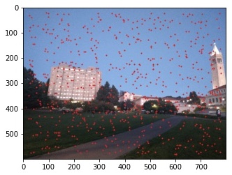
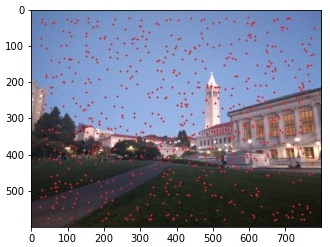
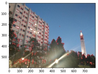
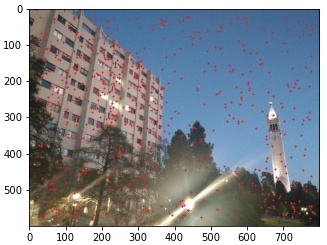
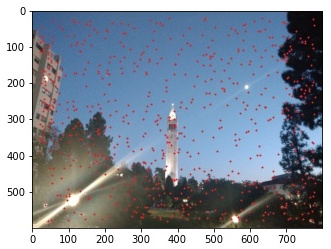
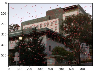
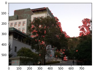
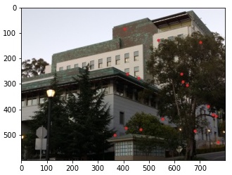
We have far too many interest points; we would like to restrict the amount to n points. Here, I used n = 700. However, if we naively select the strongest n features, they will be clustered along edges, resulting in a poor distribution of points. In order to obtain points with a better distribution, we use Adaptive Non-Maximal Suppression (ANMS). ANMS computes a suppression radius for each point (which is the smallest distance to a neighbor that is significantly stronger.) The strongest feature thus has a suppression radius of infinity. Afterwards, we can sort the points by suppression radius and take the top n points. Now, instead of getting the n strongest features, we get the n most dominant in their region.
Below shows the comparisons between the naive method and the ANMS method.

For each feature point, we sample a 40x40 pixel patch around the point and downsample it to a 8x8 patch. Then, we bias/gain normalize the patch by subtracting it by the mean and dividing by the standard deviation.
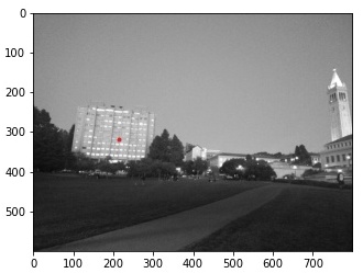
The following shows one of the feature points and its feature descriptor patch. We would need to do the same for all feature points to extract all the descriptors.


Now that we have the feature descriptors for each image, we want to match them and create correspondences. Using only SSD to compare patches may result in an undesirably high percentage of incorrect matches, as shown in the graph below. Therefore, we will use Lowe's trick, which thresholds the ratio of the SSD of the closest match and the SSD of the second closest match. Conceptually, we assume that there is only one correct match for each feature, so we reject matches that have similar first- and second-best errors and only keep matches in which the best SSD error is significantly better than all other errors.
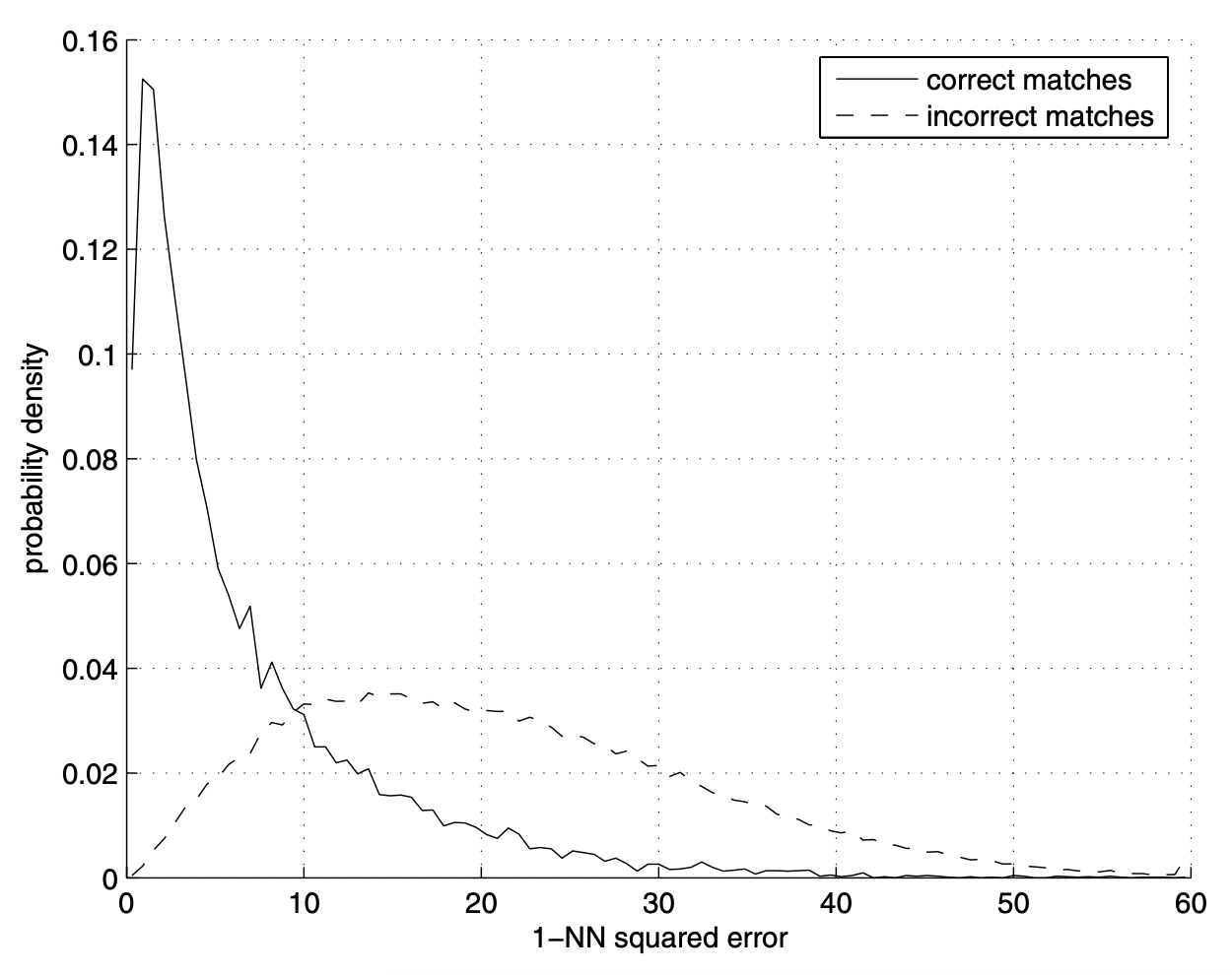
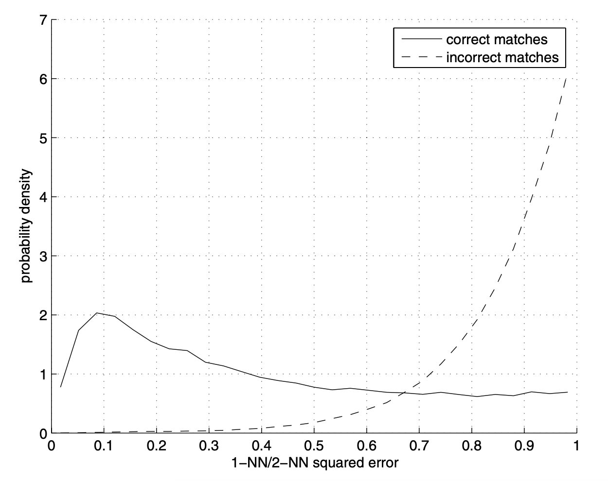
Figures by Brown, Szeliski, Winder
For the following images, I used Lowe's trick with a threshold of 0.3.

Matching features with Lowe's trick may still produce incorrect matches (i.e. outliers), so to compute a robust homography, we turn to RANSAC (Random Sample Consensus).
RANSAC randomly chooses 4 points in the source image and computes a homography.
Then, the homography is applied to each source feature point and compared to its corresponding destination feature point.
If the distance between the points is under some threshold epsilon, this match is considered an inlier and we keep it.
We loop through this process n times, and at the end, we take the largest set of inliers and recompute a homography.
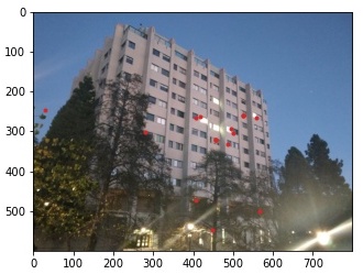
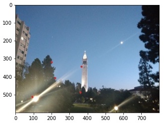
I used n = 10,000 steps and epsilon = 1 pixel. Below are the results.


With our RANSAC homography, we can now warp and blend the images into a mosaic. The warping and blending procedure is the same as that in Part A.
I did however make one change to masking. Keeping with the theme of automated mosaic-stitching, I wanted to be able to use the same mask for all photos instead of creating unique alpha channel masks for each photo as I did in Part A. As shown below, the alpha channel mask feathers the edges so that the image is more transparent near the image borders. Although this made the image masking process faster and easier, the resulting mosaic borders are not as sharp as those in Part A.
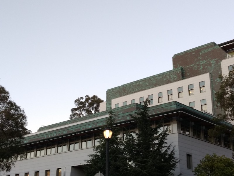
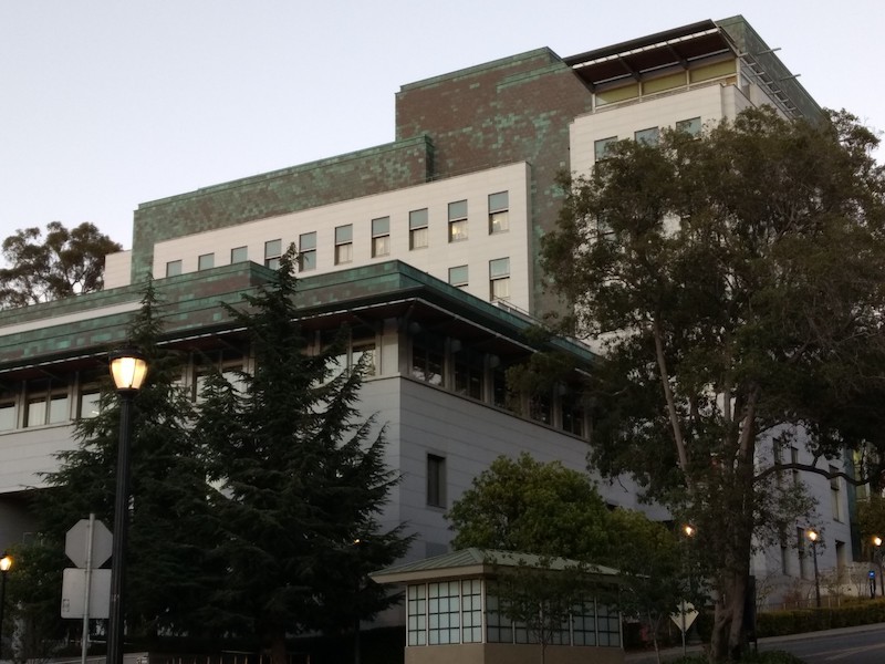
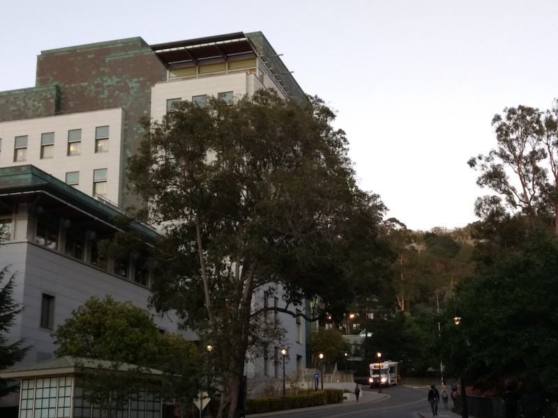
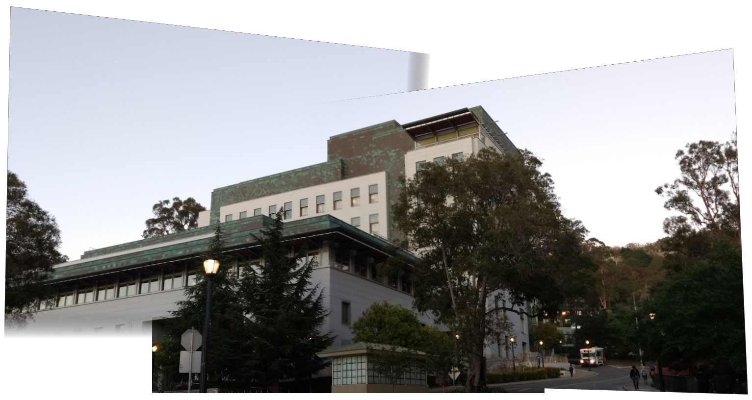
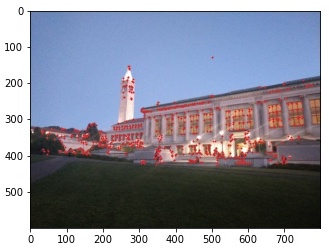
Here are some additional mosaics using the automated feature matching method.


Automatic feature detection and matching makes stitching mosaics a lot easier and is more precise than manual correspondence selection.
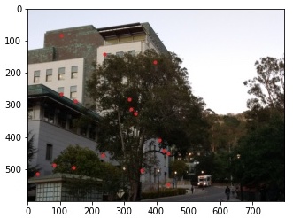
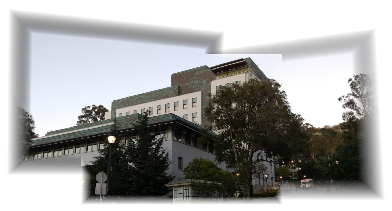
But, I did notice that the automatic method works better for images with buildings (like Stanley Hall which has many sharp corners and details)
than images with lots of even textures (like the Memorial Glade photos which contain a lot of sky).
Again, the blending and alpha channel masking can still use improvement.
Ideally, I would like to retain sharp mosaic borders but also prevent harsh lines in the interior of the mosaic, which can be achieved through 2-band blending.
Overall, although implementing part of a research paper was challenging, it helped me better understand the concepts and the motivation behind each step.