Hi! This project explores using homographies to stitch images together.

In the first part of the project, I focus on computing the homographies need to stitch two images into a mosaic. Here, we manually define the correspondences used to compute the homography.

In the second part of the project, I follow the “Multi-Image Matching using Multi-Scale Oriented Patches” research paper by Brown et al. in order to automatically extract image corrrespondences. From there, I use the RANSAC algorithm to define matching points and then compute the homography used to stitch the images together.

 

Project Part 1

1.1: Shoot and Digitize Images

1.2: Recover Homographies

1.3: Warp the Images

1.4: Blend the Images into a Mosaic

 

Project Part 2

2.1: Detecting Corner Features in an Image

2.2: Extracting a Feature Descriptor for each Feature Point

2.3: Matching these Feature Descriptors between Two Images

2.4: Using RANSAC to Compute a Homography

2.5: Compare the Auto-Correspondence and Manual-Correspondence Mosaics

 

What I Learned

A reflection on the key learnings through this project.

 

1.1: Shoot and Digitize Images

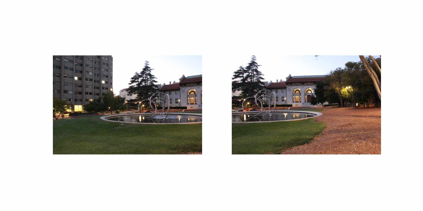
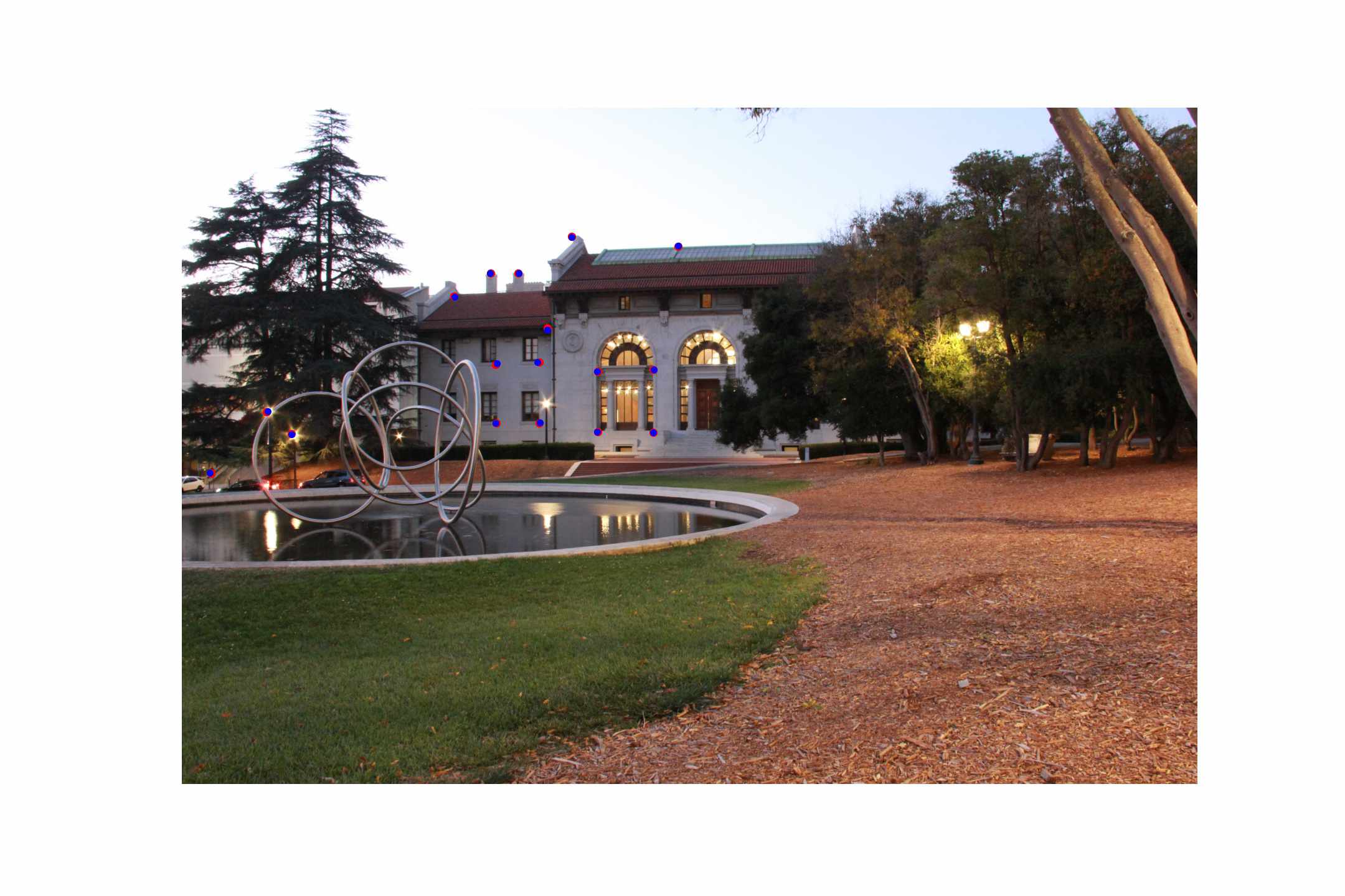
The first task was to shoot images that have overlapping correspondences. I chose to use a DSLR camera and shoot images with some friends in the class. We shot photos around campus-- in a library, by Heart Mining Circle, and by the campanile. As it got darker, the images were more difficult to shoot, but we made it work by adjusting the aperture and exposure.

To initially develop my code, I used the following images of Hearst Mining Circle.

 

1.2: Recover Homographies

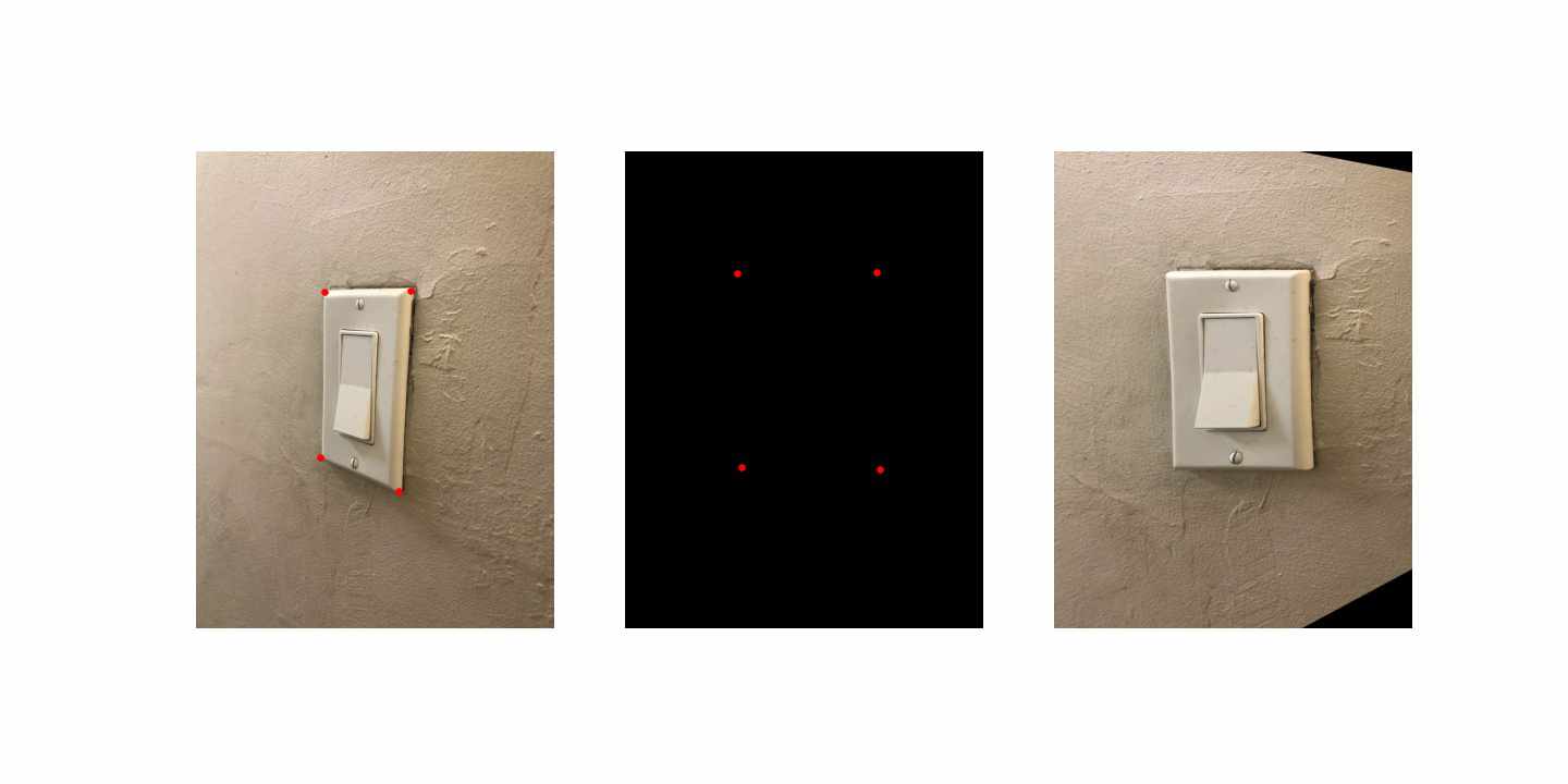
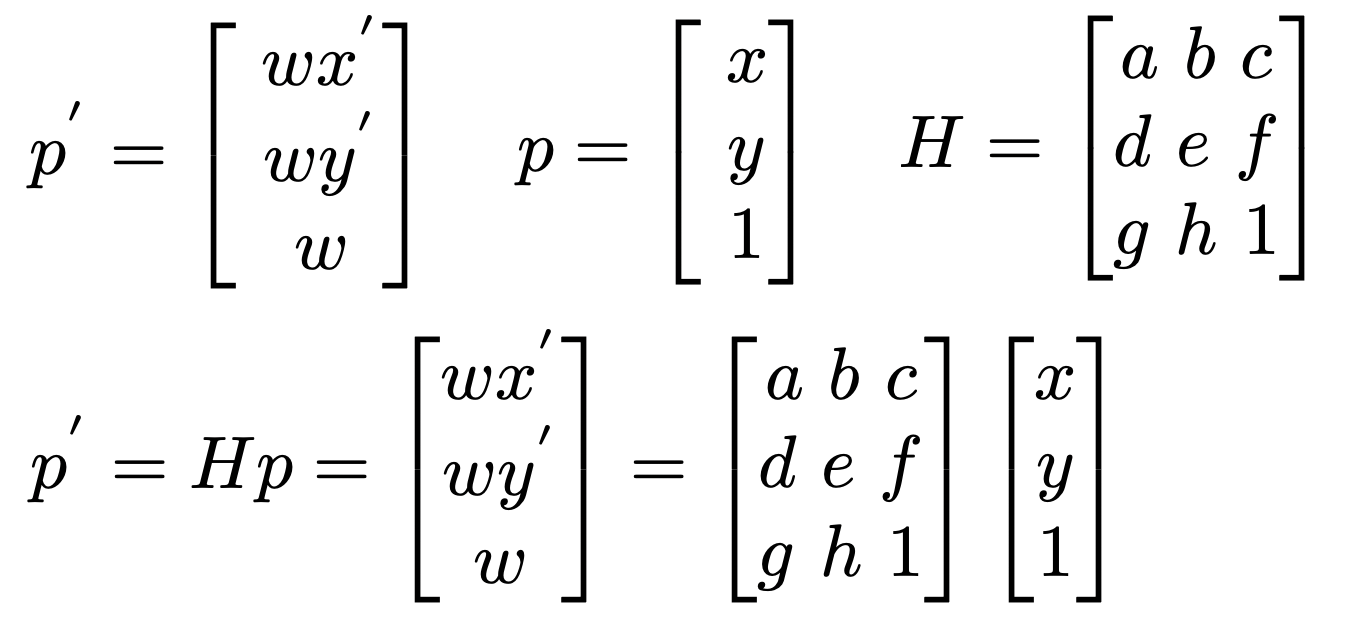
To start, I needed to recover the 3x3 transformations between the two images. This would transform coordinates in the first image to the plane of the second. The 3x3 transformation matrix applies a homography, such that p' = Hp, as shown below. There are 8 unknowns within the equation, so 4 points is enough to specify the homography. However, because we're specifying the correspondences by hand, these homographies are prone to error. Instead, we formulate the problem using Least Squares, and solve for the H matrix values that minimizes error.

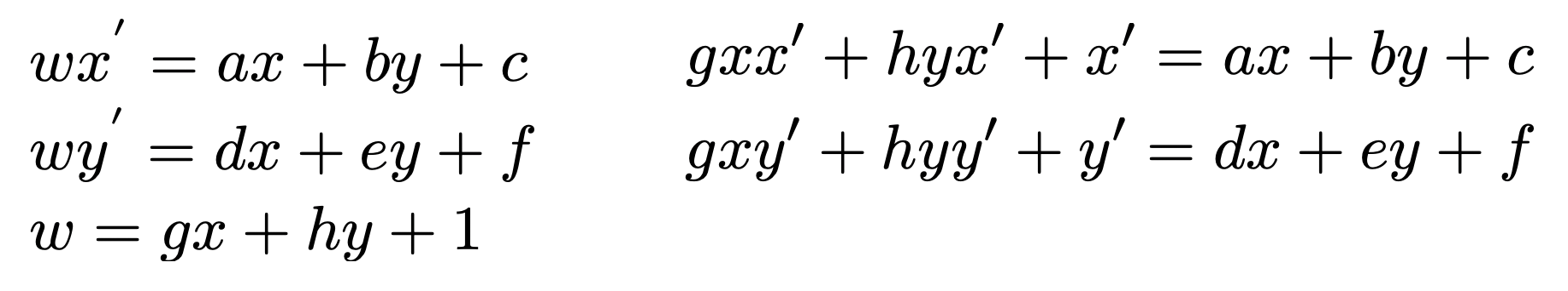
We can write out these equations and rearrange them such that all our unknowns are in an 8x1 array. The equations below illustrate the equation for 1 pair of corresponding points. For more, we would simply vertically stack a repetition of the b and A arrays.

I tested whether the homographies worked by transforming the correspondence points using my calculated homography matrix. We can see that the points overlay each other-- not perfectly, but well enough.

 

1.3: Warp the Images

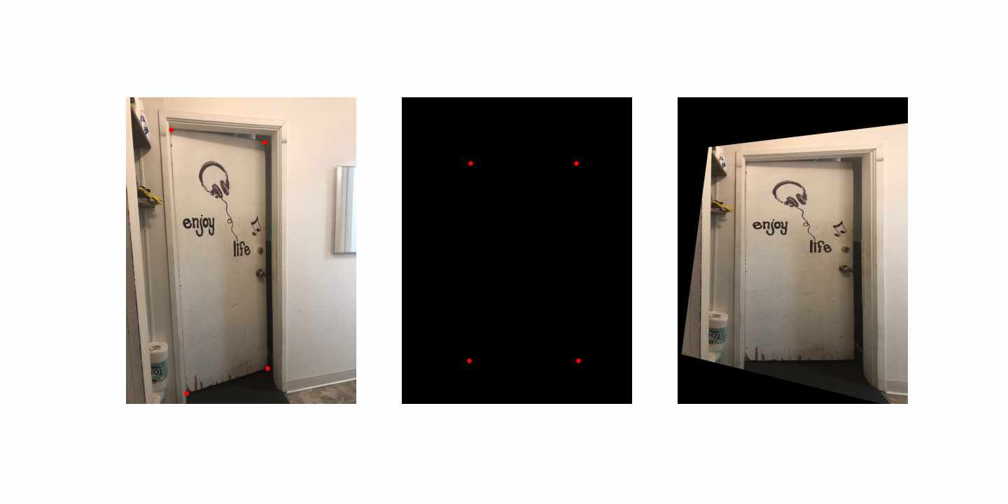
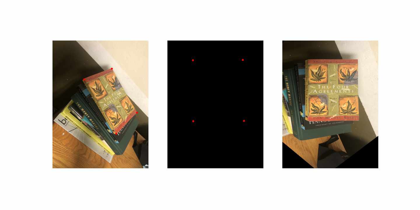
Next, I wrote a function to warp all the points of one image into the plane of another. The function takes in the two images and the homography between them. It first applies a calculated pad that is found by transforming just the corners of the second image using H's inverse. From there, I know exactly where the second image will land in the plane of the first image. I can pad the first image accordingly-- although because of rotations in the image, this pad results in some of the warped image being clipped sometimes.

The warp function uses cv2.remap, looking up values of the new warped image from the second image. First, I tested this on some images that had a known rectangular shape when viewed from the front. This allows me to check that my warp function works as intended before testing it on two images in arbitrary planes. The results work fairly well, although there's some details that look a bit odd. For example, from the stack of books, we can see the sides of the stack of books that were visible in the first image, even though we wouldn't expect to be able to see these if we were truly viewing from the top. The reason for that is that truly viewing the book from the top requires us to move our viewing point, which is impossible after we've captured an image.

 

1.4: Blend the Images into a Mosaic

Finally, I took two images, warping one to the plane of the other. I used an alpha mask to stitch the two images together, which sets the overlap of the two images to 0.5 and the unique parts of their masks to 1. This allows me to multiply each image -- the original padded one and the new warped one-- by the alpha mask, taking a average of values for just the overlapping region.

The results are shown below! We see that there is quite a bit of blur within the overlapping regions, which is attributed to error in selecting correspondence points. This gets worse for the darker images, which already have an inherent blur that makes it difficult to classify the points. In the next part, I'll improve on this by automatically detecting correspondences.

 

Hearst Mining Circle

     

Library Books

     

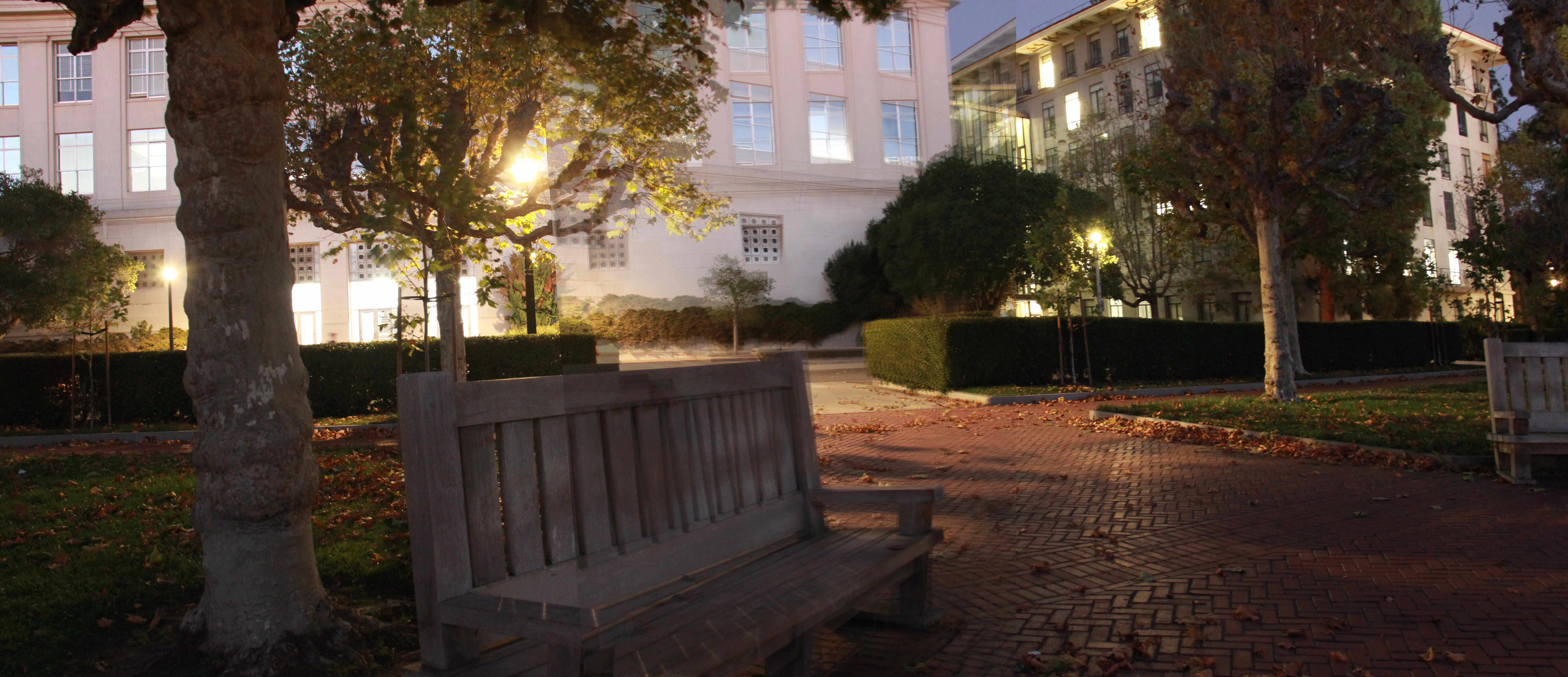
Campanile Benches

     

2.1: Detecting Corner Features in an Image

Harris Corner Detection

In this part, I implement the correspondences matching technique shown in “Multi-Image Matching using Multi-Scale Oriented Patches” by Brown et al., but with several simplifications. We start by detecting the Harris corners in each image, which detect variations in any direction within a window. We see that initially, we have many identified corners.

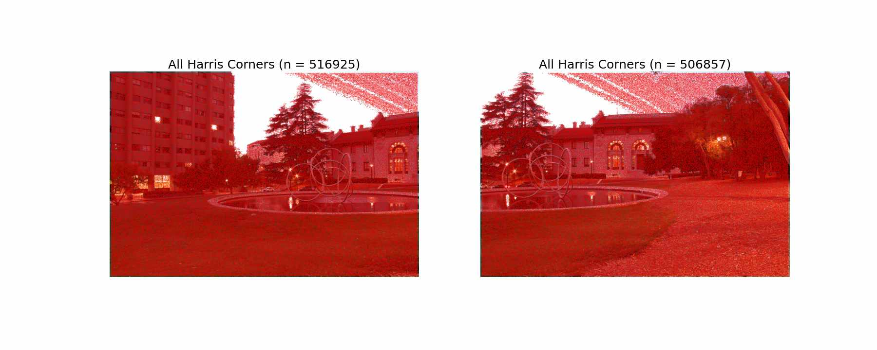
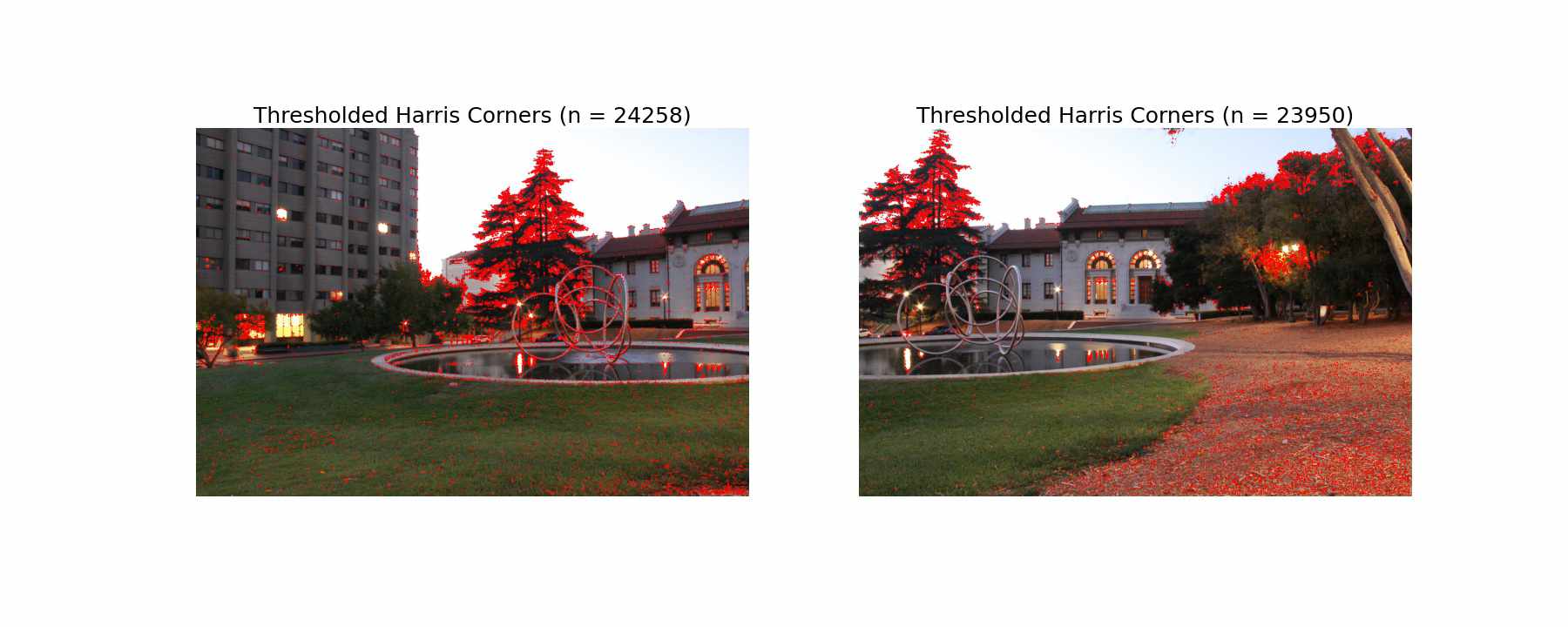
Each point is given a corner score, which we can use to threshold the amount of Harris corners we compute on. Although we might be losing some correspondences, this will greatly speed up our computations for the next step.

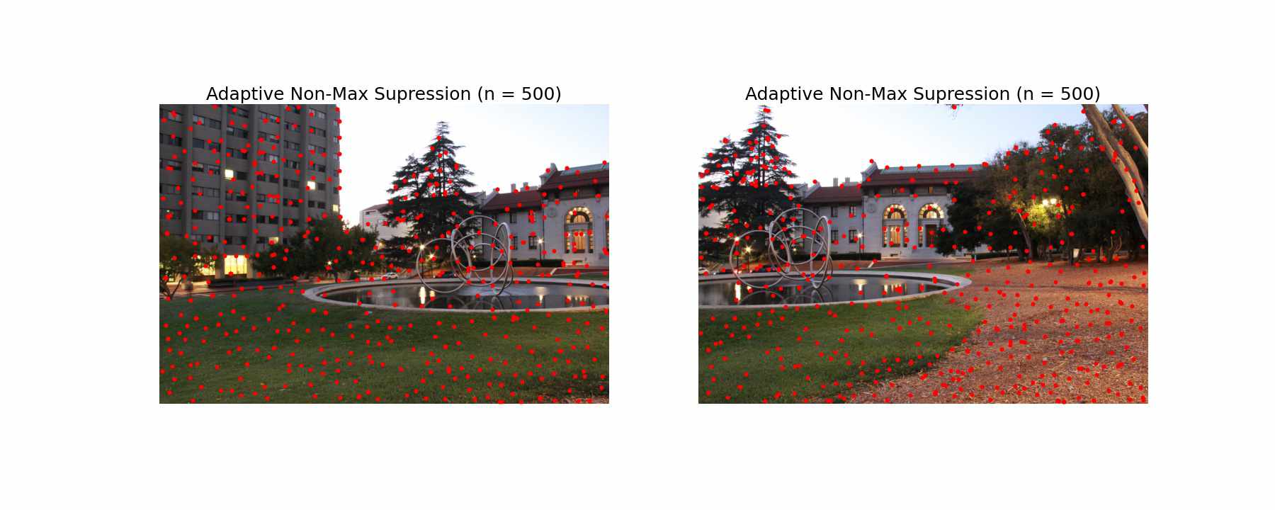
Adaptive Non-Maximal Suppression

Next, we perform Adaptive Non-Max Surpression (ANMS), as described in the paper. The purpose of this is to find corners that are distributed throughout the image evenly, as the initial Harris Corners tended to be concentrated in higher frequency areas of the image. For example, we have a lot of points in the tree, which likely isn't a great correspondence because it could shift in the wind.

To implement ANMS, for each point, we assign a radius that tracks the closest neighbor such that point_corner_score < c_robust * neighbor_corner_score. I used the hyperparameter suggested in the paper, defining a neighbor's corner score to be sufficiently larger when c_robust = 0.9. From there, we can order our list by descending radius, and only keep the top n points. For my algorithm, I used n = 500.

 

2.2: Extracting a Feature Descriptor for each Feature Point

Next, we take 40x40 patches around our chosen Harris corners after adaptive non-max suppression. We downsample these patches, only taking every 5th pixel in order to create 8x8 feature descriptors for every point. To implement this, I used np.mgrid, spanning the desired window around the point. Some example patches are shown below.

 

2.3: Matching these Feature Descriptors between Two Images

Next, we want to find the matching feature descriptors between the two images. In order to do this, we employ a similarity index, namely SSD. Since we are left with 500 points in each image after ANMS, we can create a 500 x 500 matrix with the SSD for each feature pair. It is difficult to set a raw error threshold for our matches, so instead, we employ Lowe's trick of ratios. The trick states that a match is more likely to be correct is the ratio of the lowest error match to the second lowest error match is low. If the ratio is closer to 1, it's not a clear correct match. Using this trick, we end up with a smaller subset of points. We still see that most of them are incorrect, but there are a few correct matches as well.

 

2.4: Using RANSAC to Compute a Homography

Finally, we use RANSAC to find the best set of points to compute a homography on. We do this by picking groups of 4 pairs of potentially matching points at random and computing a homography. From there, we test the error for every pair of correspondences using that computed homography. Those that fall within an error bound are added to our inlier set. The remaining are outliers. We reason that the largest set of inliers are matching points. In order to find the best fit homography, we finish by taking this largest set of inliers and recomputing our homography using Least Squares as we did in the first part of the project.

 

2.5: Compare the Auto and Manual Correspondences