Project 4: Autostitching Photo Mosaics
COMPSCI 194-26: Computational Photography & Computer Vision (Fall 2021)
Alina Dan
4A: Image Warping and Mosaicing
Shoot the Images
Here are the pictures I shot and used for this project:
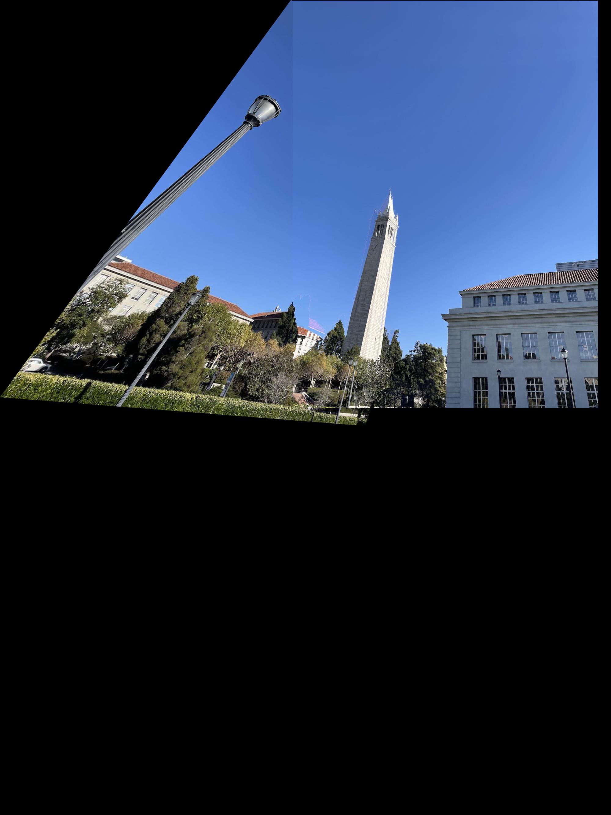
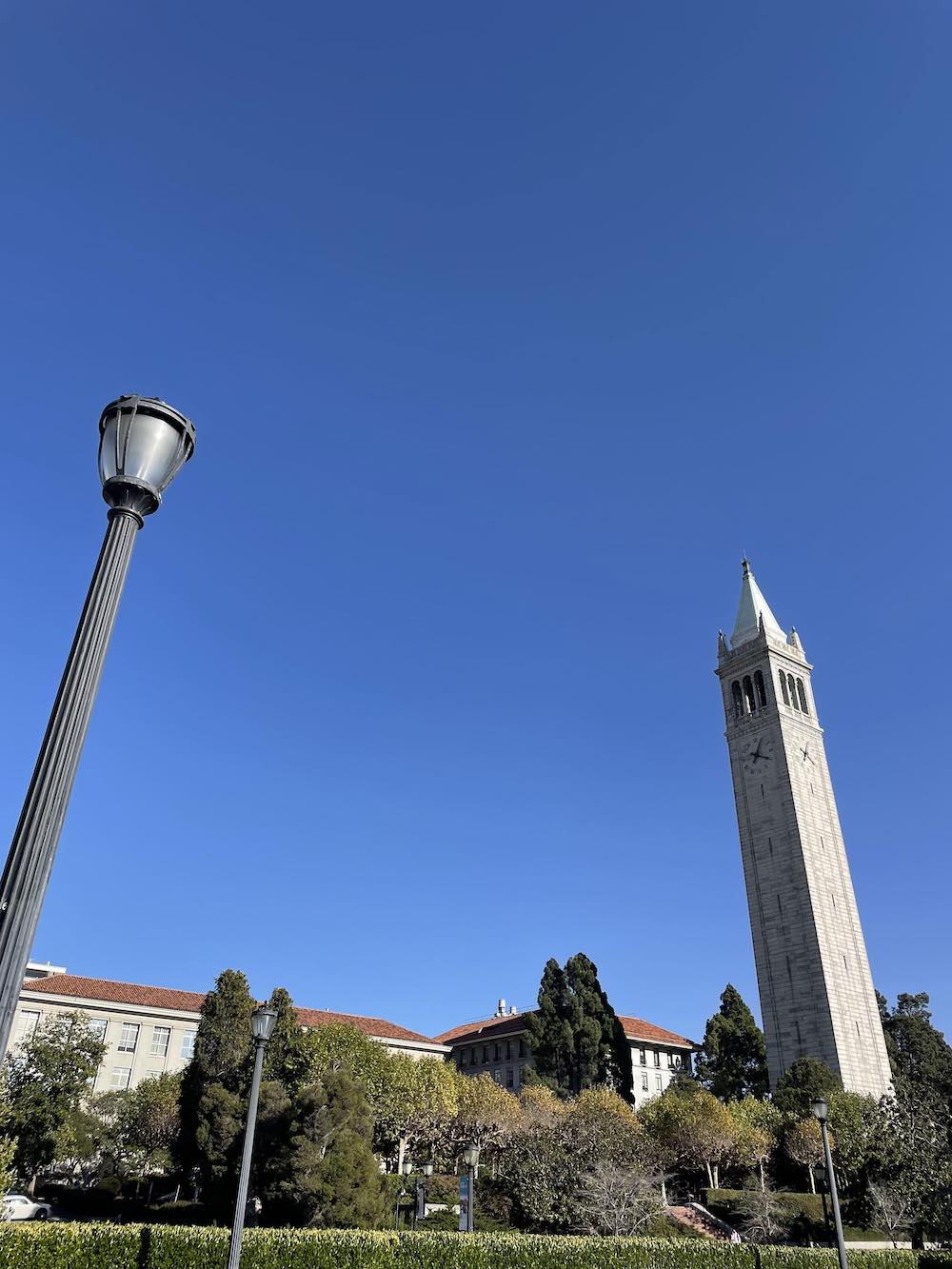 Campanile Left
|
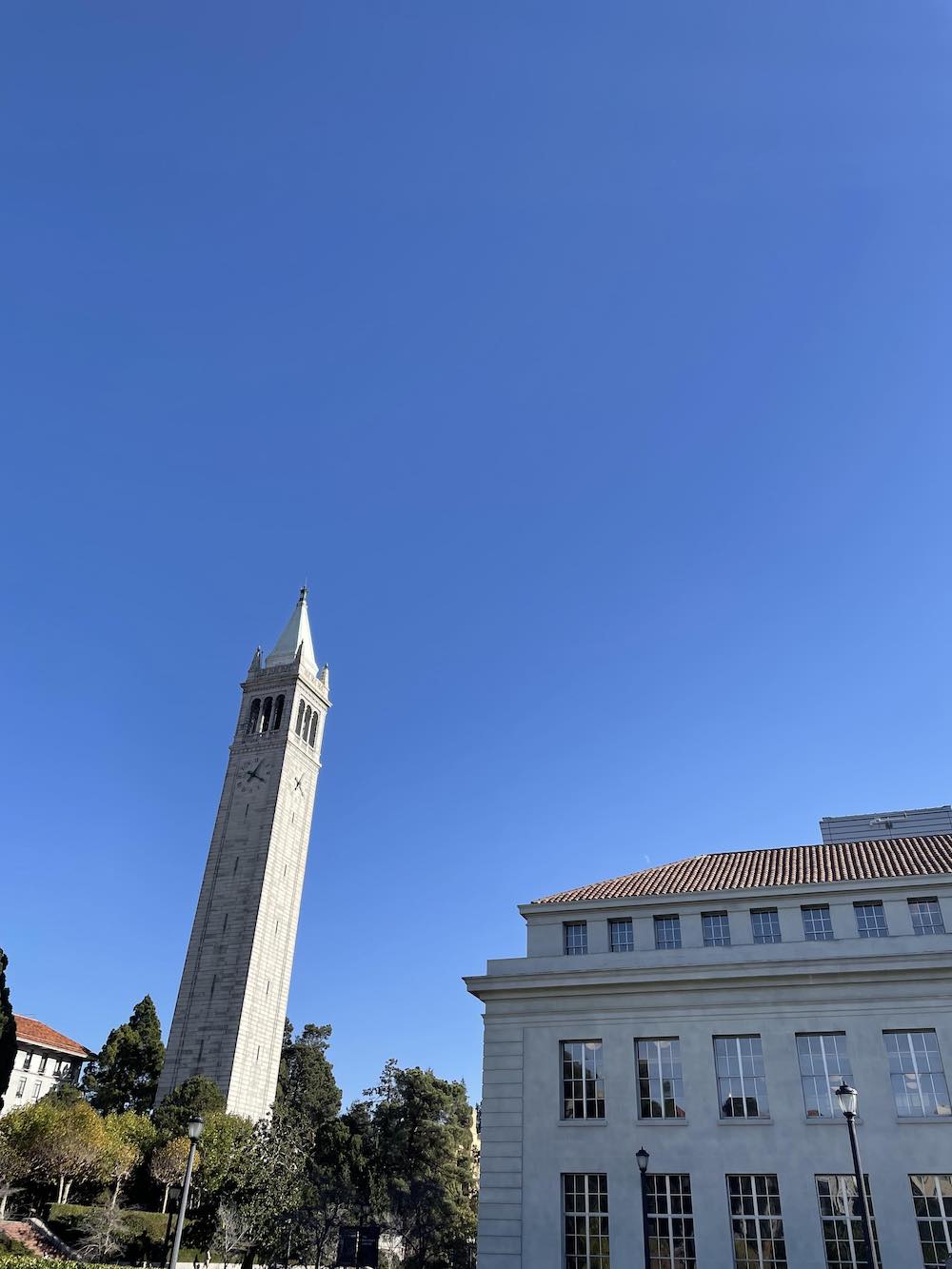 Campanile Right
|
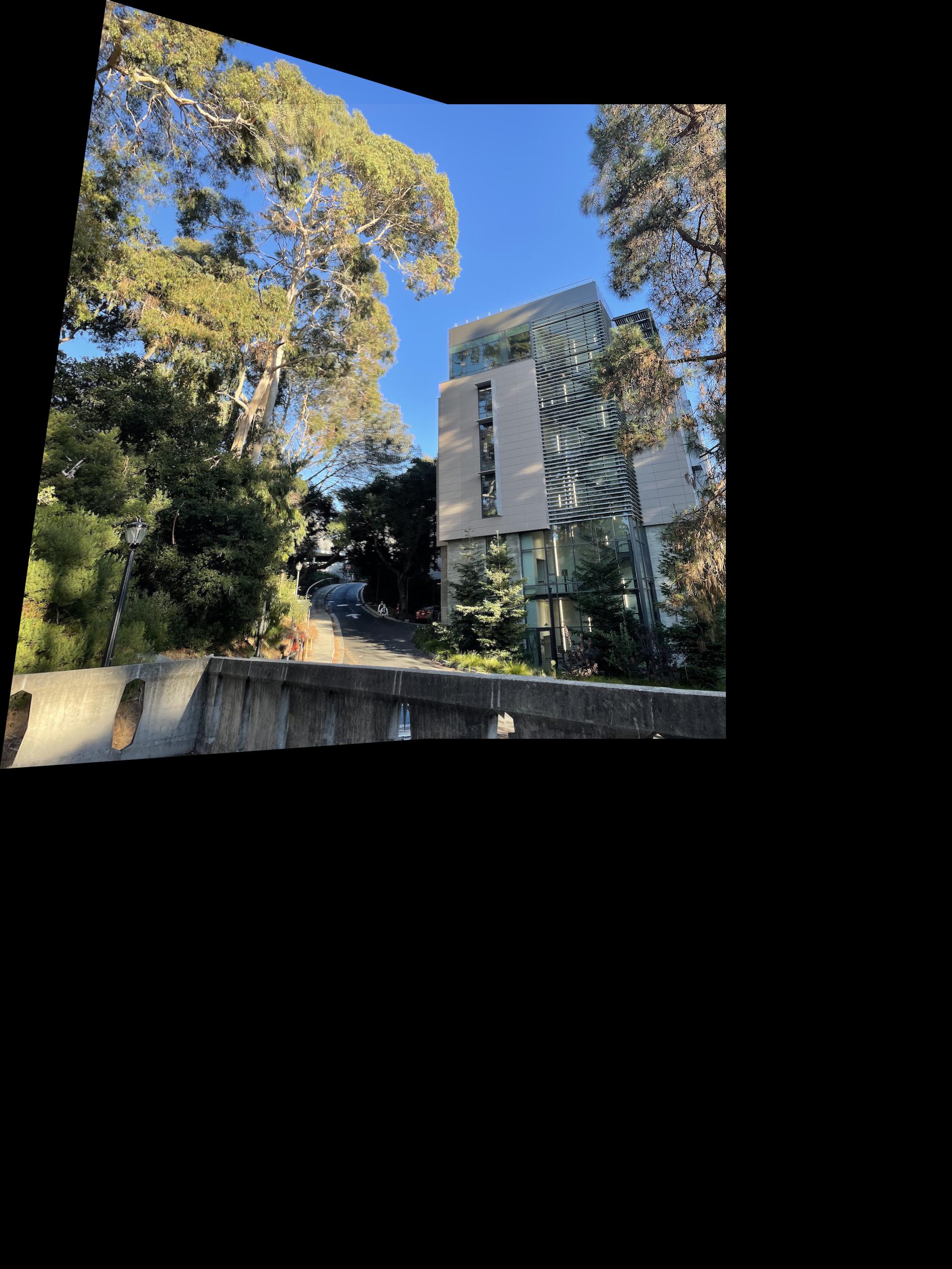
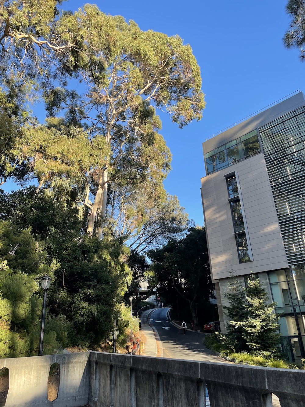 Outside Lewis Left
|
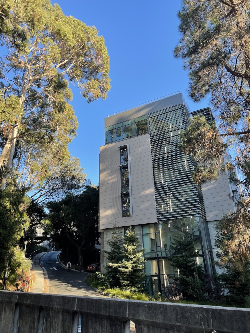 Outside Lewis Right
|
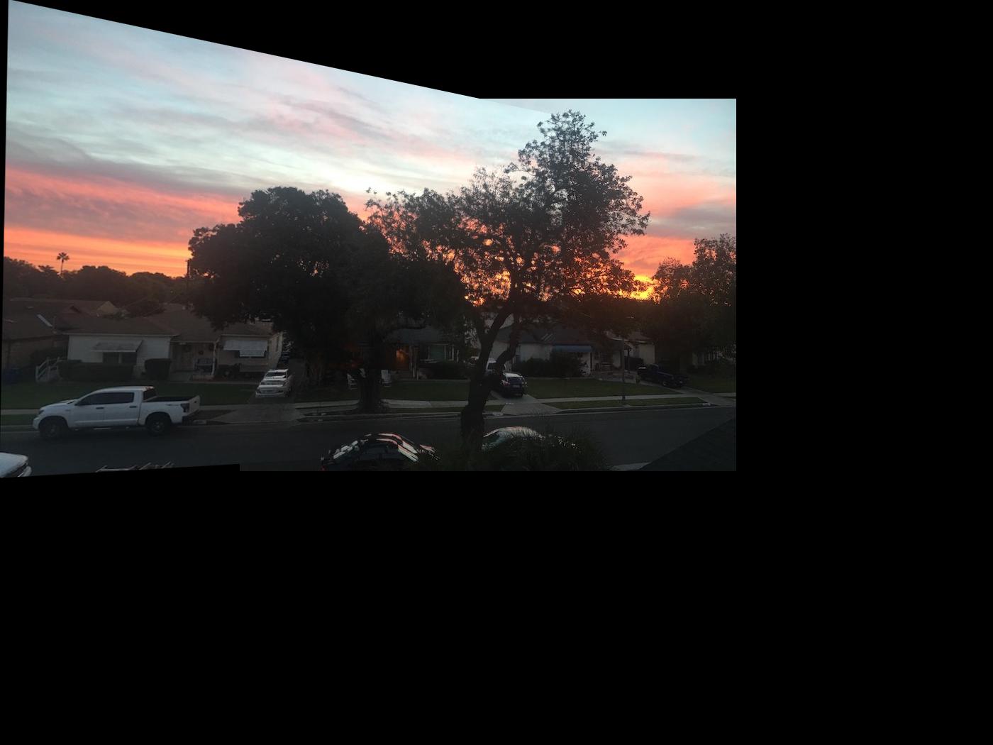
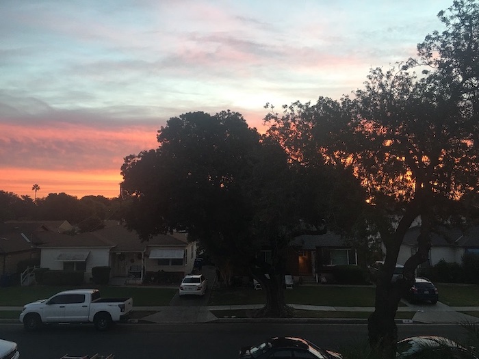 Sunrise Left
|
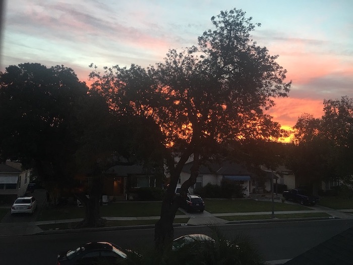 Sunrise Right
|
Recover Homographies
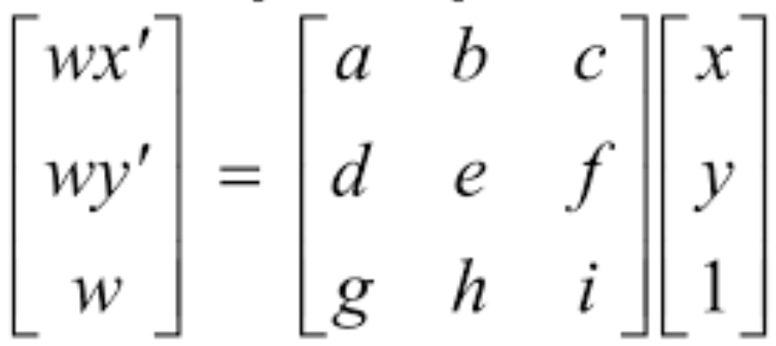
To find the transformation between one image to the other, I found the homography based on correspondence points from both images. I did this by utilizing the formula, p' = Hp:
|
Each correspondence points results in two equations, and to recover the homography, at least 8 equations are needed. Thus, at least 4 correspondence points are required; however, more points are better to combat noise and unstableness. With the data points, I used least squares to solve for the H matrix.
Warp the Images
After recovering the homographies, I did image warping for rectification. This was done with inverse warping and interpolation based on 4 corners of an image like so:
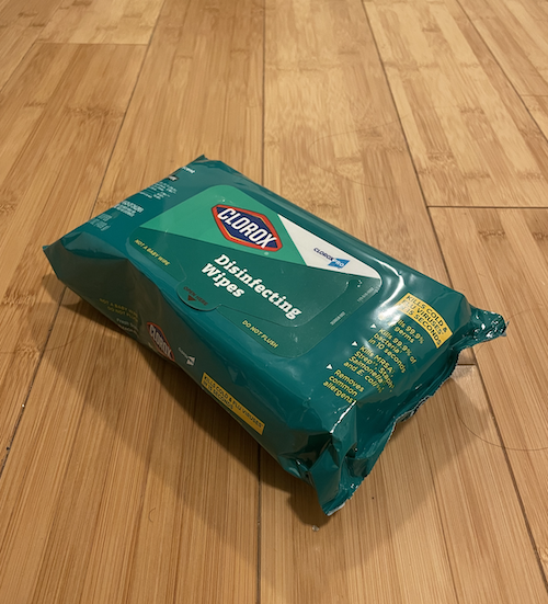 Wipes
Wipes
 Rectified Wipes
|
 Book
Book
 Rectified Book
|
Blend the Images into a Mosaic
After ensuring my recovering of homographies was working well, I went on to actually blend picture together to form a mosaic. By warping images such that they are in the same plane, I can align them based on their correspondence points. This then allows for creating of a mosaic / panorama picture like so:
|
Campanile Left
|
Campanile Right
|
 Campanile Mosaic
|
|
Outside Lewis Left
|
Outside Lewis Right
|
 Outside Lewis Mosaic
|
|
Sunrise Left
|
Sunrise Right
|
 Sunrise Mosaic
|
Learnings
The most important thing I've learned from this part is the complexity revolving around picking the "right" pictures. For some of the images I tried to rectify or warp into a mosaic, the algorithms and code didn't work too well. I had to retry with other images due to noise and other issues that caused the rectification and blending to not work so well. I have learned that for computer vision, the pictures that you choose really play a huge role into the outcome.
4B: Feature Matching for Autostitching
Harris Interest Point Detector
Using the provided code for detecting Harris corners, we found potential correspondence points. Trying it on one of my images from the former part, this is the result:
 Lewis Left with Harris
|
 Lewis Right with Harris
|
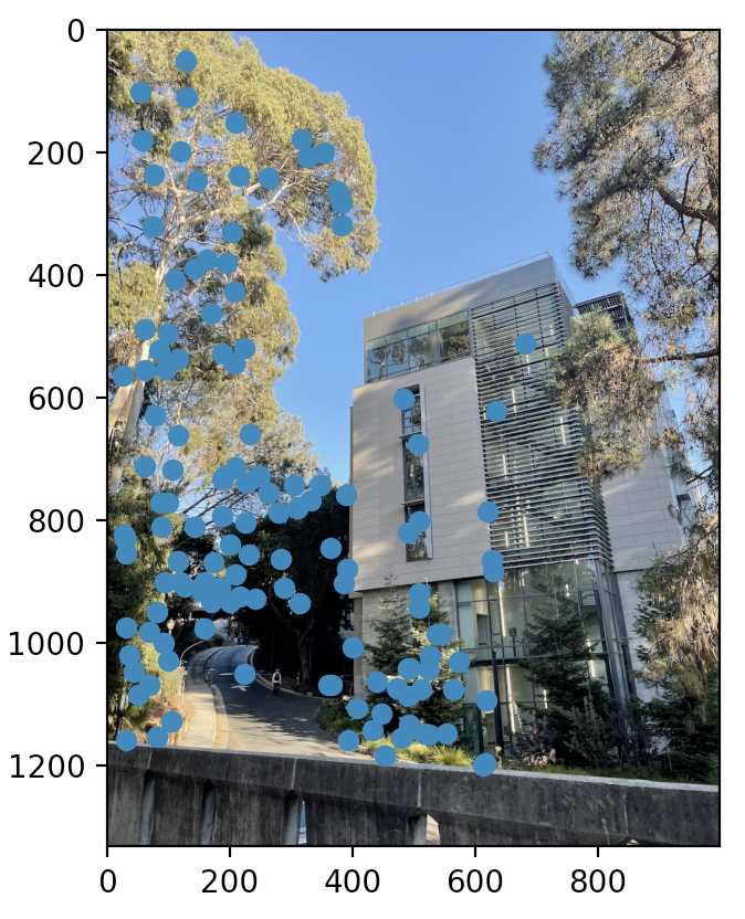
Adaptive Non-Maximal Suppression
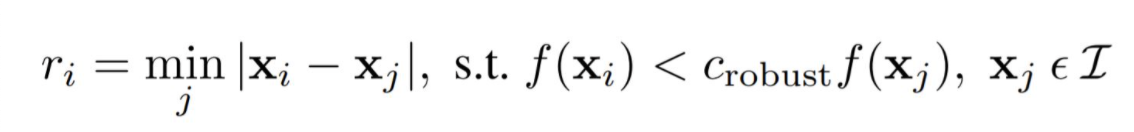
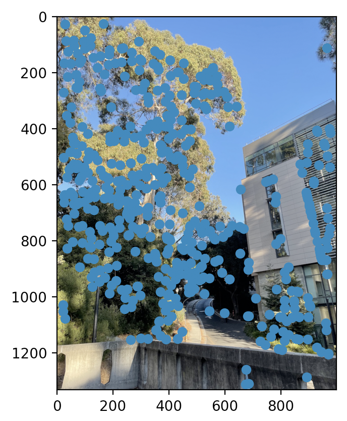
Because of the great number of points detected with the Harris Interest Point Detector, I went on to use Adaptive Non-Maximal Suppression (ANMS) to filter through the points. The basis of ANMS is to filter points out such that the correspondence points are pretty uniformly distributed throughout the image. For my implementation, I filtered the points such that I was left with 500 points based on this formula:
|
For this algorithm, we calculate the minimum suppression radius for each of our potential correspondence points, sort the points by that radius (descending), then keep the top X points where X in this case was 500. That resulted in filtering like so:
 Lewis Left with ANMS
|
 Lewis Right with ANMS
|
To further filter through the 500 points, I extracted feature descriptors from our images. For each of the 500 points, we look at a window of 40x40 pixels surrounding the point, Gaussian blur it, then downsample it to a window of 8x8 pixels. Following this, we normalize the patch by ensuring we have a mean of zero and a standard deviation of one.
For each of the patches from the previous section, I computed the sum of squared differences (SSD) between a patch in one image and the patches in the other image. I kept track of the smallest (1-NN) and second smallest (2-NN) SSD values for that particular point. With these values for each of the patches, I computed the ratio between them: 1-NN / 2-NN. Only correspondence points with a ratio less than that of a threshold (.6 in my case) were kept--others were discarded.
RANSAC
For this section of the project, I implemented the RANSAC algorithm:
- Select four feature pairs (at random)
- Compute homography H (exact)
- Compute inliers where dist(p_i, H p_i) < ε (ε = 5 pixels)
- Keep largest set of inliers
- Re-compute least-squares H estimate on all of the inliers
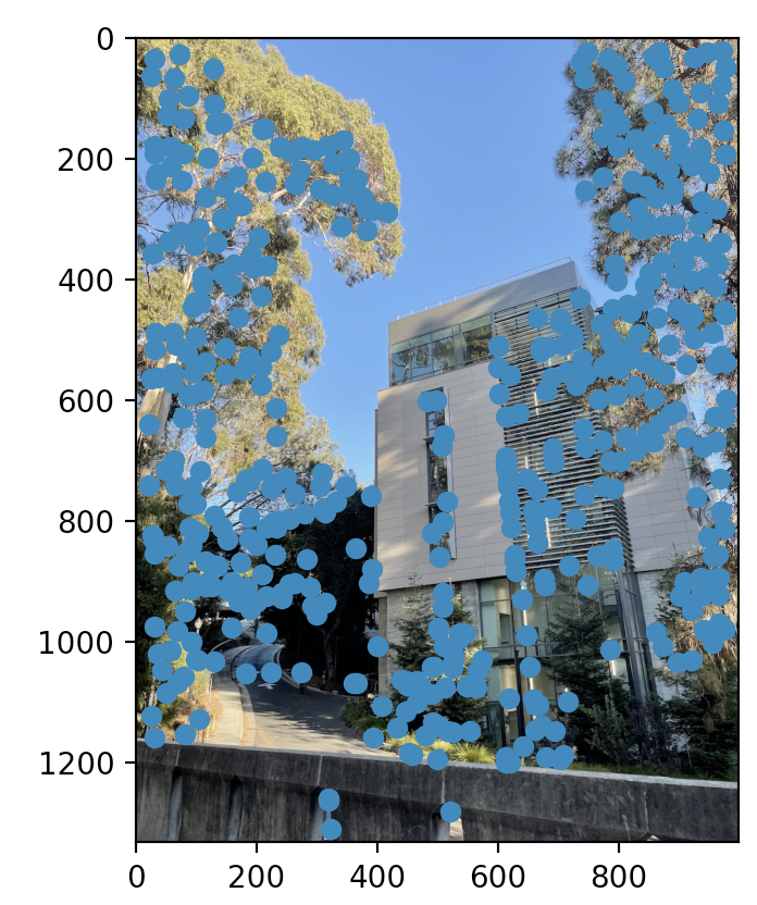
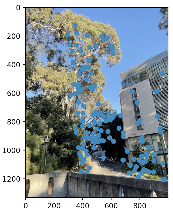
This allows for computing an appropriate homography while continuing to filter out points attempting to minimize the number of outliers in our data. These are the correspondence points left after all the processes listed above and the RANSAC algorithm:
 Lewis Left with RANSAC
|
 Lewis Right with RANSAC
|
Mosaics
Here are the results of the filtering, inverse warping, and blending. I've included on the left side, the results from part 4A, and on the right, the results from part 4B.
|
Lewis Mosaic 4A
|
 Lewis Mosaic 4B
|
|
Campanile Mosaic 4A
|
 Campanile Mosaic 4B
|
|
Sunrise Mosaic 4A
|
 Sunrise Mosaic 4B
|
Learnings
The coolest thing I learned from this project was the intricacies related to automating the process of choosing correspondence points (along with filtering) and how that affects mosaicing. The fact that there are many algorithms to help facilitate this process (ex. ANMS and RANSAC) and their powers was really eye-opening and fun to learn about. It was also really interesting to see how manually picking correspondence points sometimes works better or worse than automated correspondence points based on the pictures being used (see the mosaics above).