In this project, we explore capturing photos from different perspectives and using image morphing with homographies to create a mosaic image that combiens the photos.
To take good photos for this project, I shot photos from the same point of view, but with different view directions, and with overlapping fields of fiew. My iPhone camera has exposure and focus locking and the photos were taken at the same time of day and location.
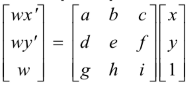
Before warping the images into alignment, we recover the parameters of the transformation between each pair of images. To do this, we are finding the homography matrix H such that p' = Hp. I computed the H matrix following the following images:
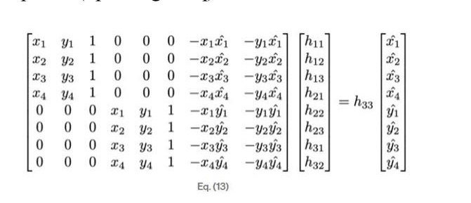
To find the homographies, I selected 6 corresponding points in each pair of images using ginput() as done in Project 3. I also verified that the homorgraphy matrix was calculated correctly through checking the values outputed by cv2.findHomography. (Red selection dots are very small on the image, sorry!)
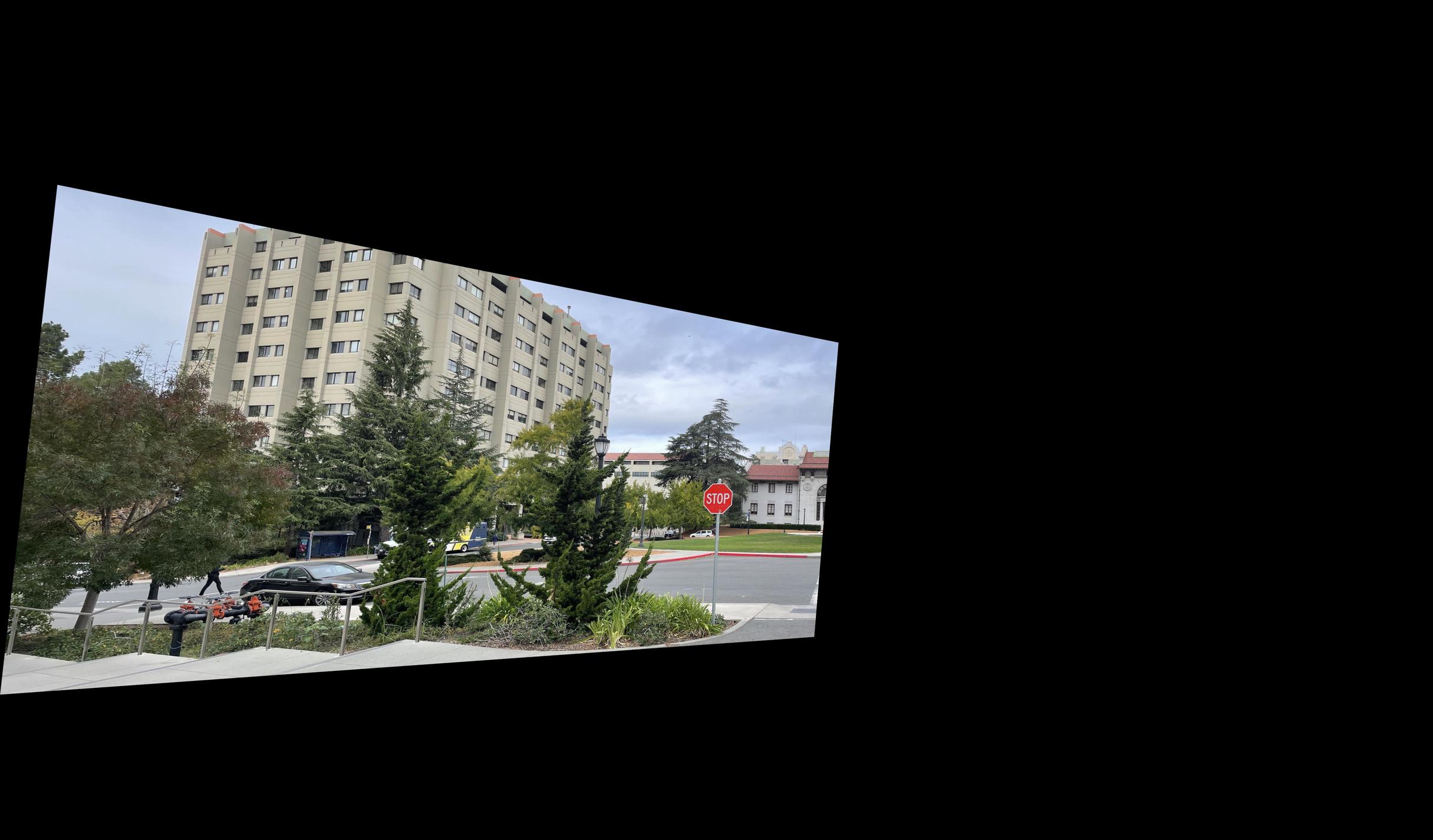
To warp the image, I used cv2.remap to map the source points of the image to the new locations. Following the documentation from this thread. The images are perpectively realigned so that theoretically, the corresponding points chosen lie directly over each other if the images were overlayed.
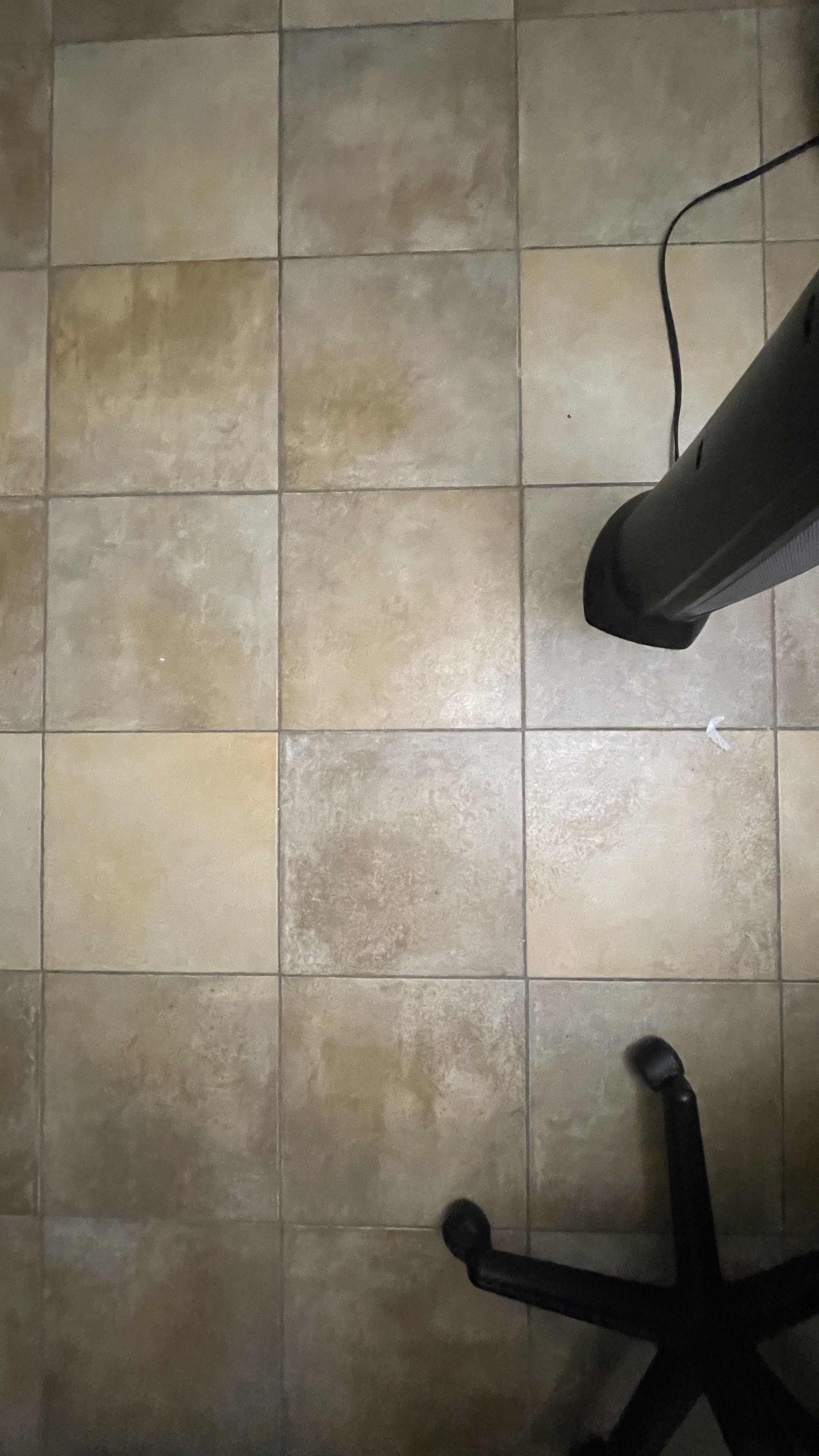
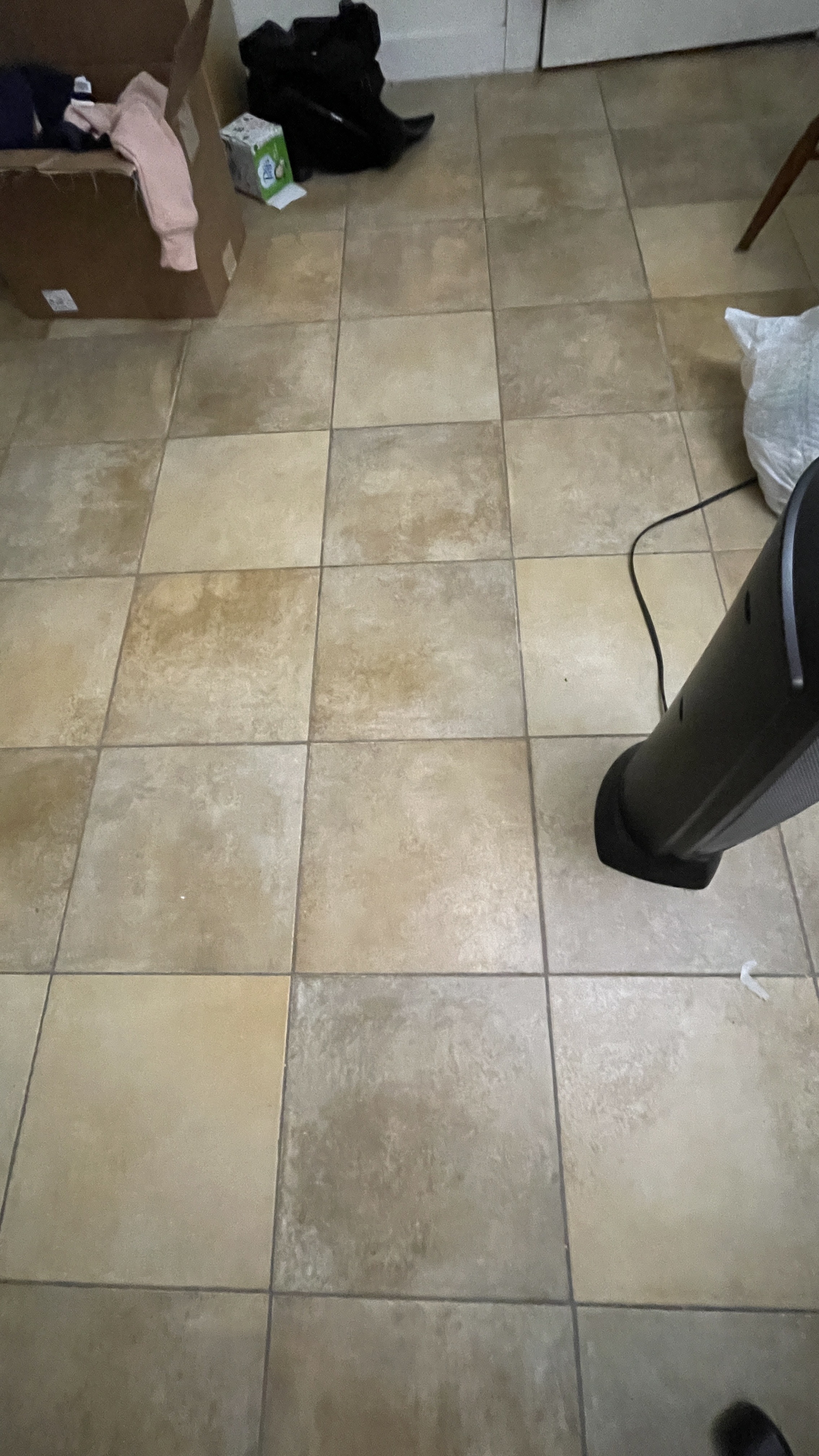
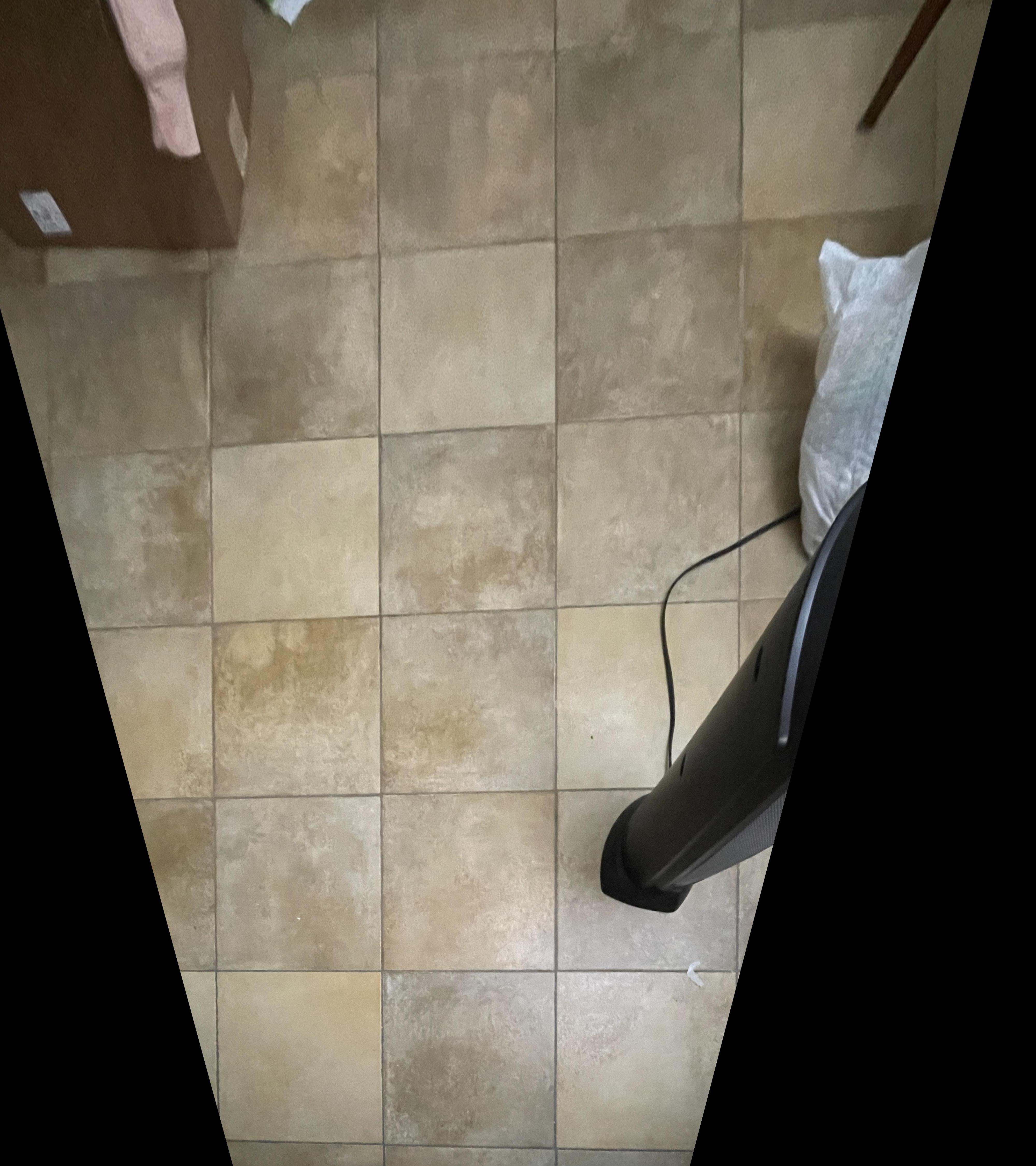
To verify my homography and warping functions, I took some sample images of planar surfaces and warped them so that the plane is frontal-parallel. I clicked the tiles of my floor and completed the same procedure as above.
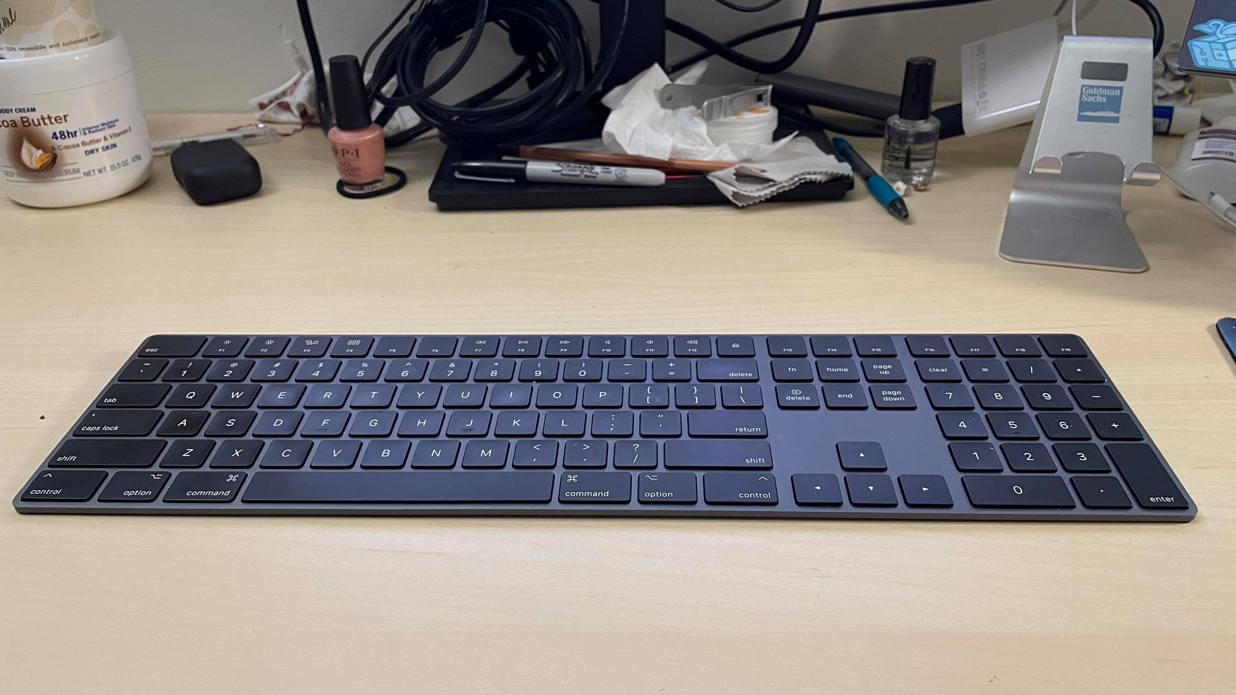
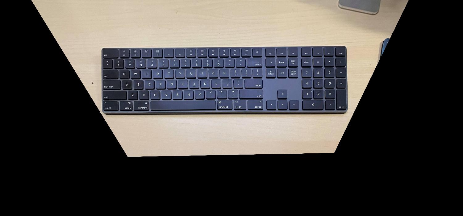
I also rectified my keyboard through picking a rectangle shape.
To blend the images into a mosaic, I warped every right image to the existing left mosaic. When blending the seams, I tried a couple different methods shown below. First, I created a mask of the intersection point and between two images, used only the intersection of one image. I called this a crude blending. Next, I tried averaging the intersection of two images. Finally, I tried getting the max pixel value of two images. While the crude blending resulted in clearer intersections, it also gave very clear lines of where the mask was found. Thus, for the rest of my mosaics, I used max pixel blending to have softer lines.
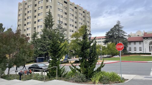
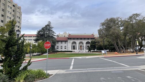
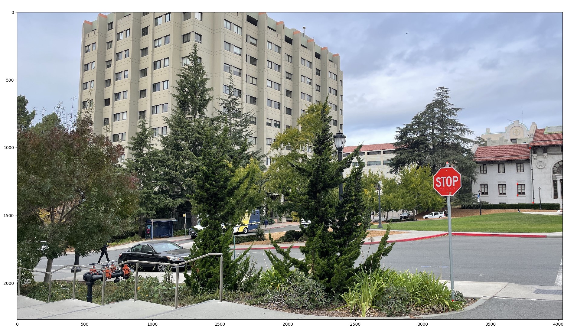
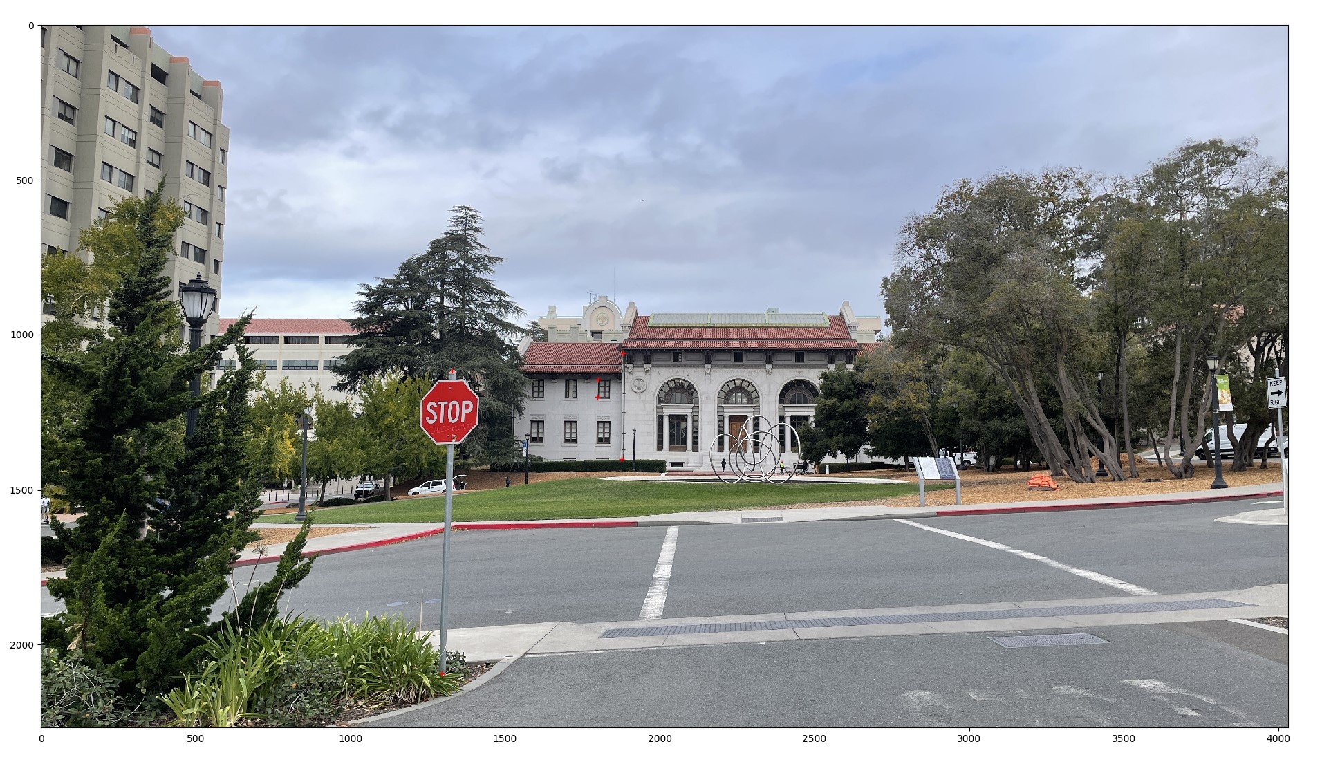
For the Hearst mosaic, below are the three images that were stiched together:
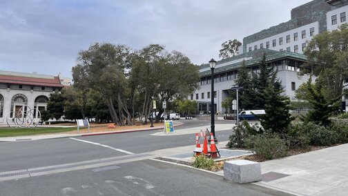
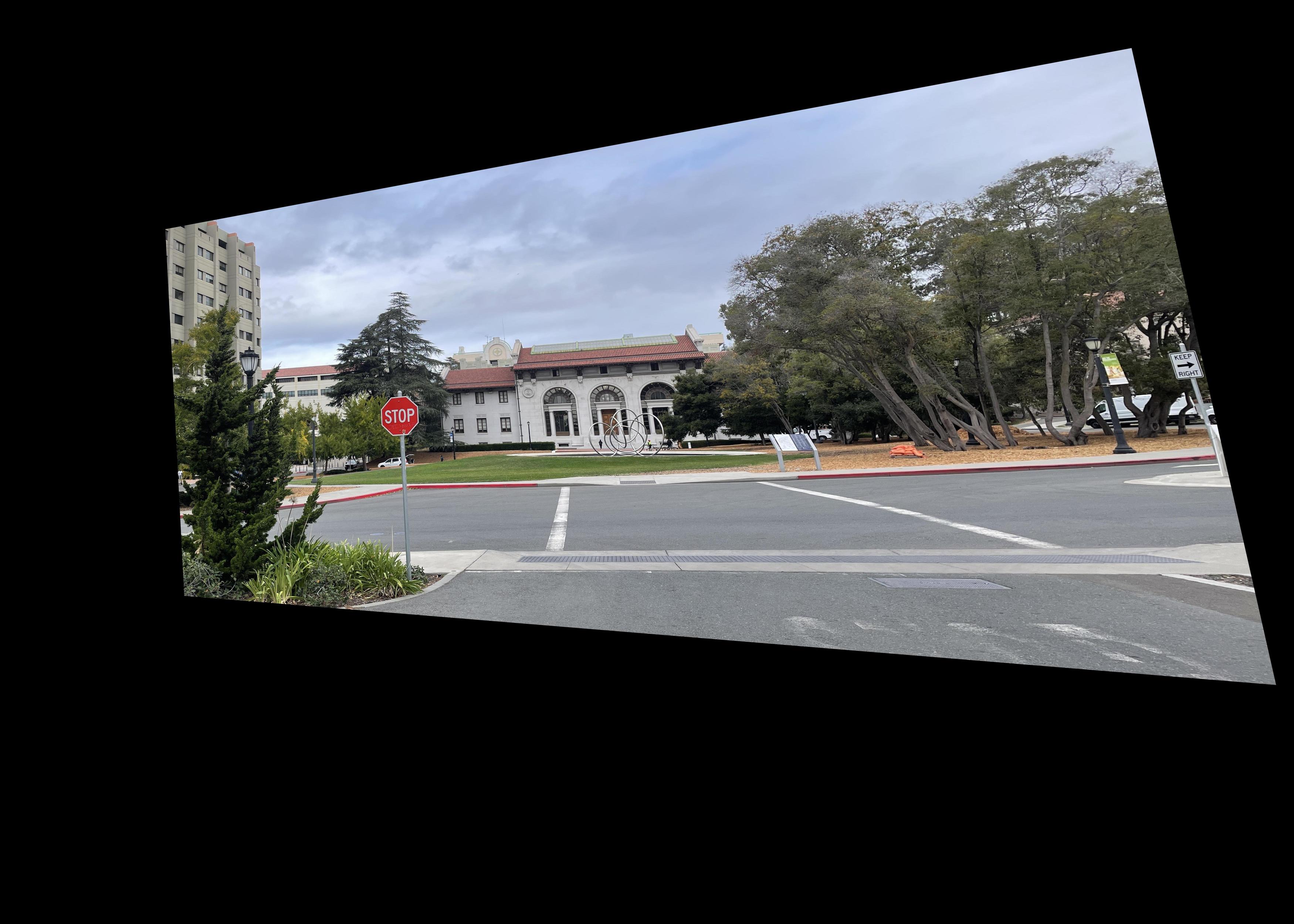
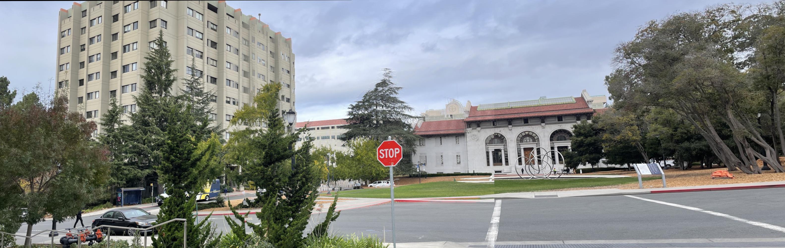
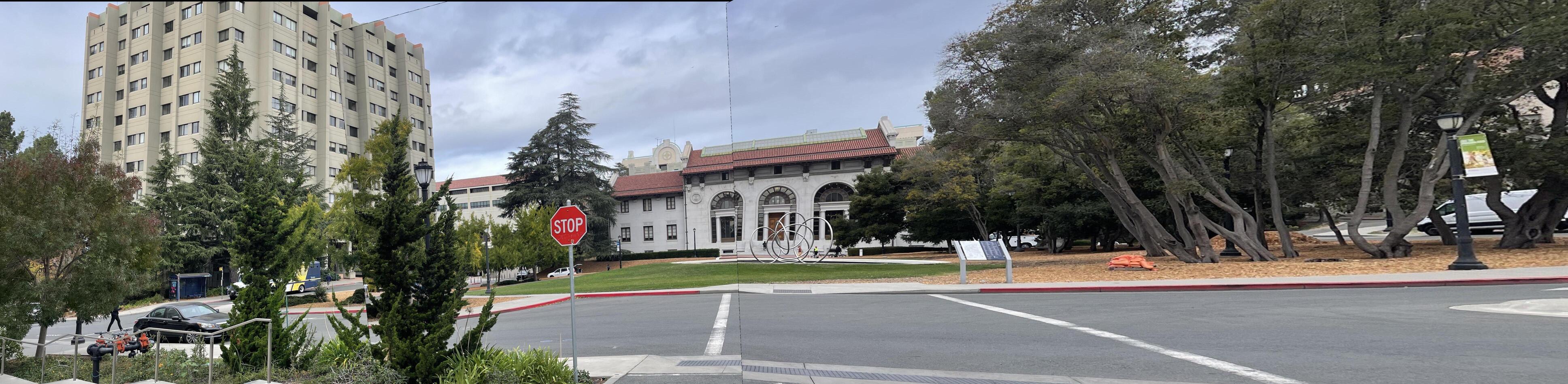
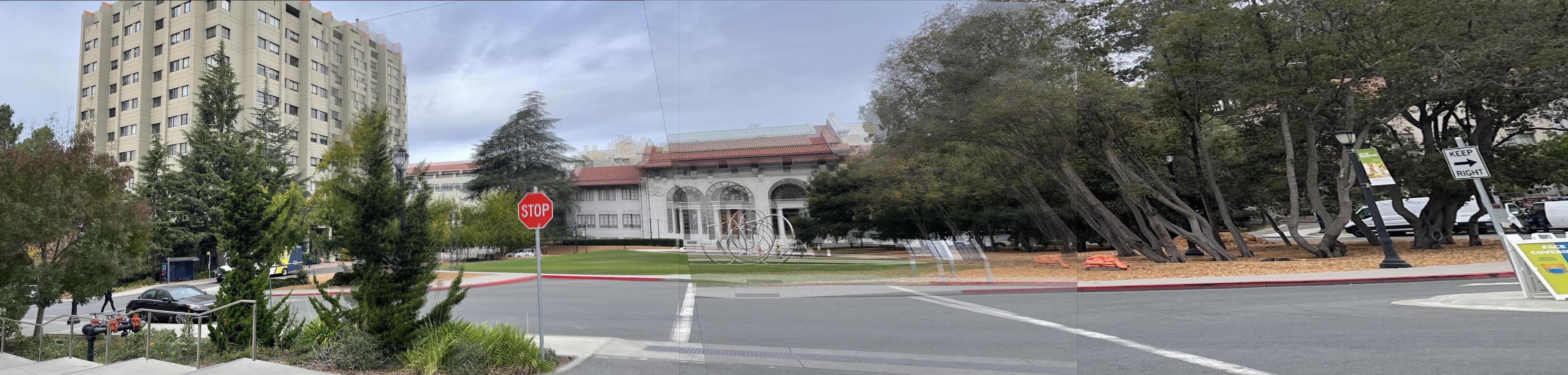
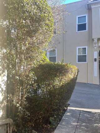
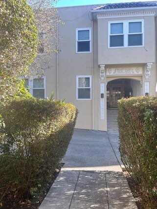
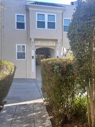
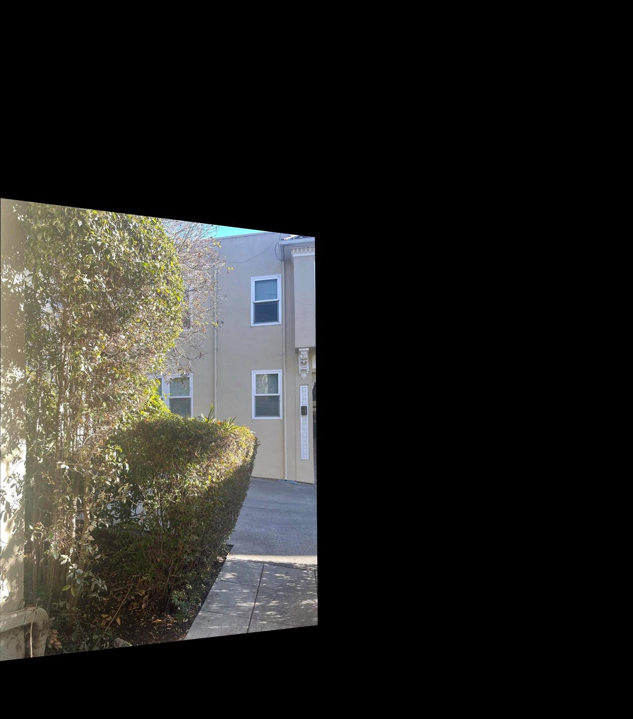
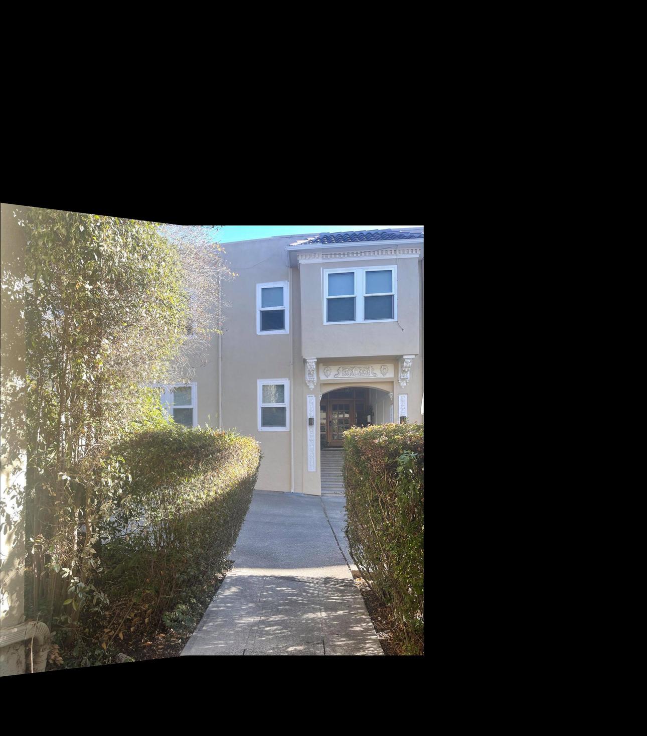
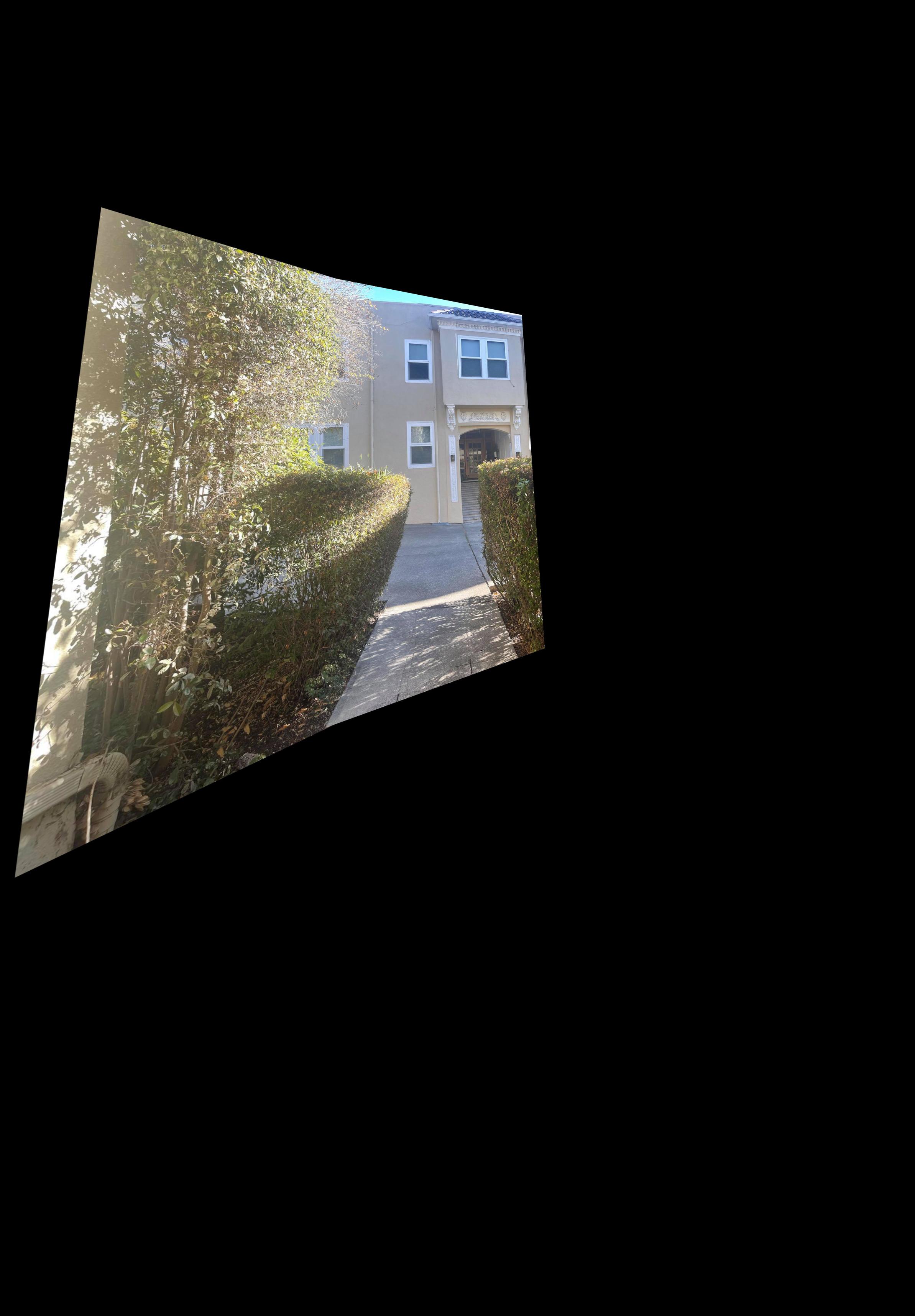
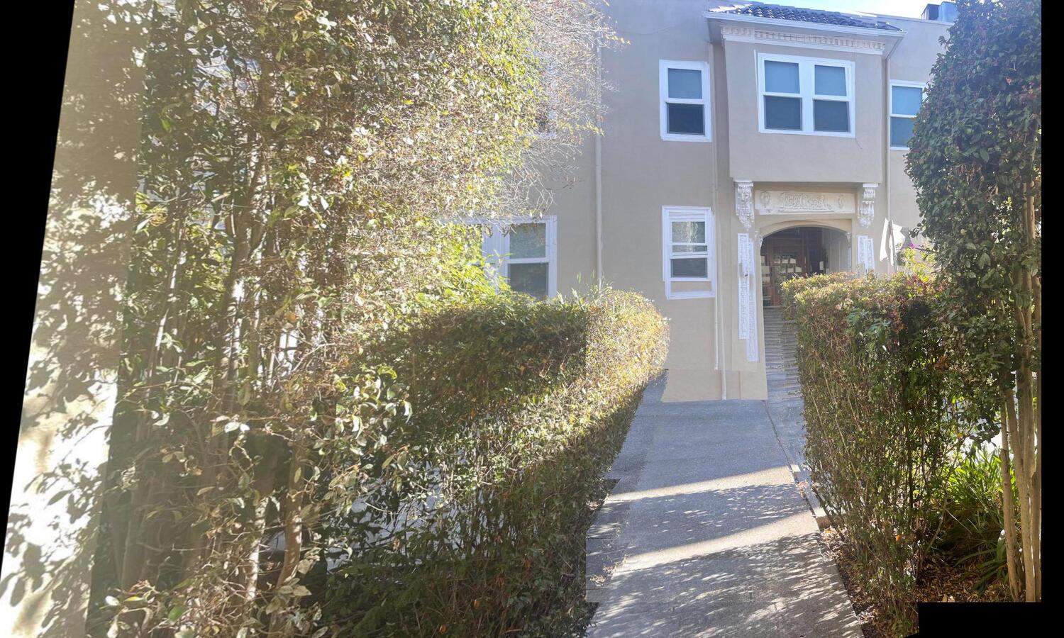
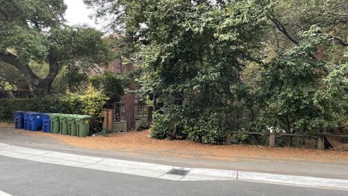
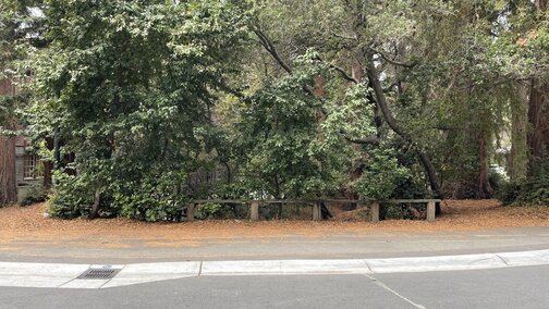
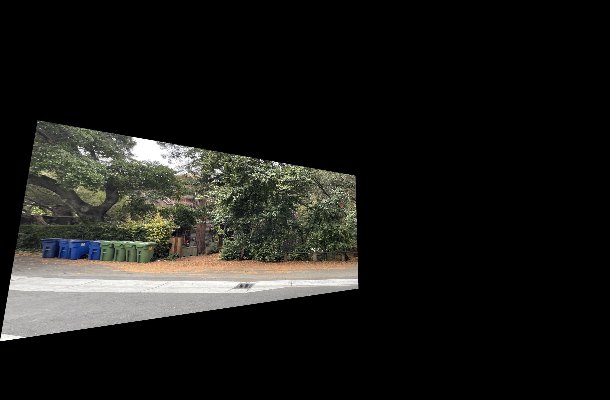
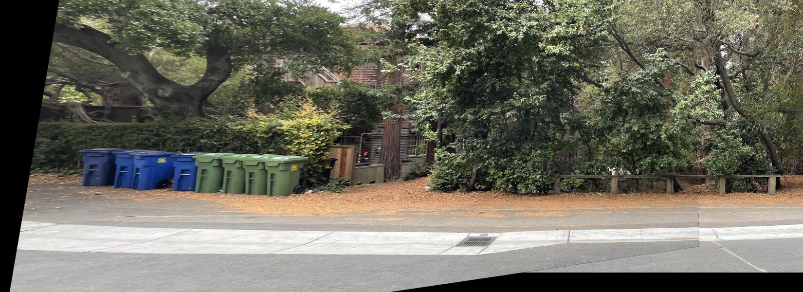
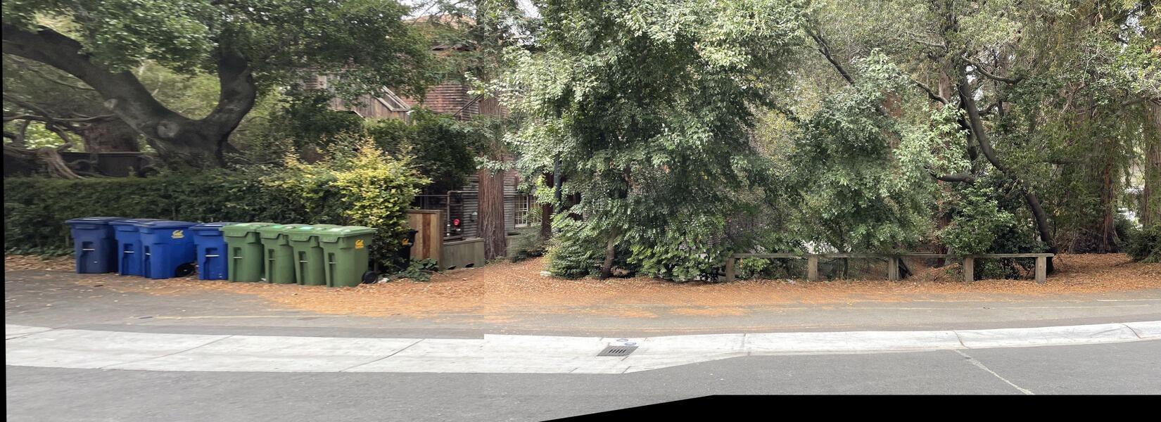
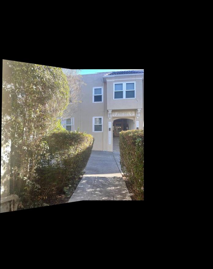
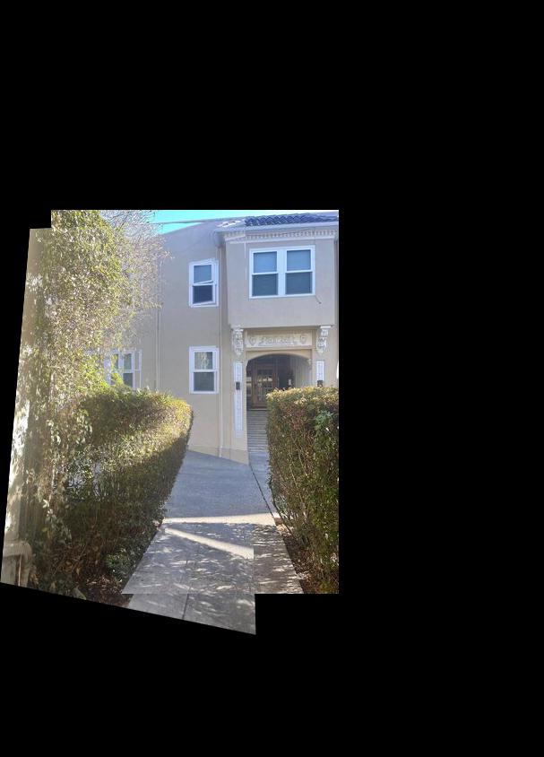
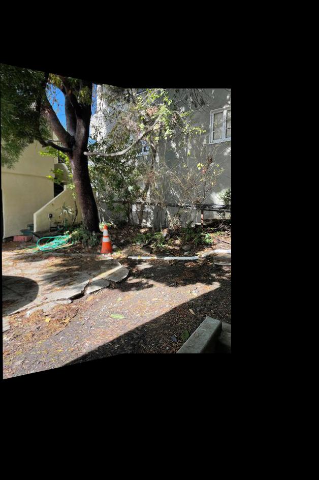
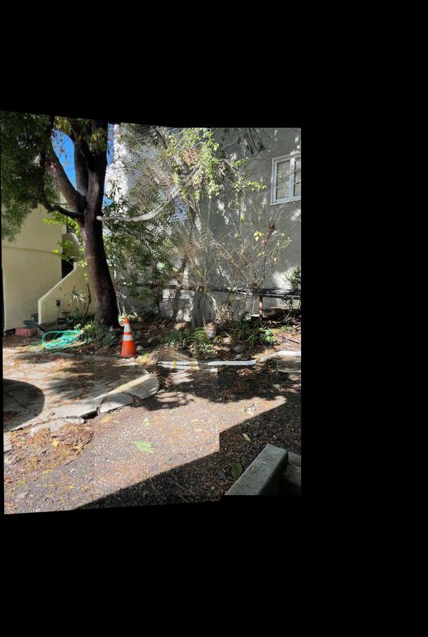
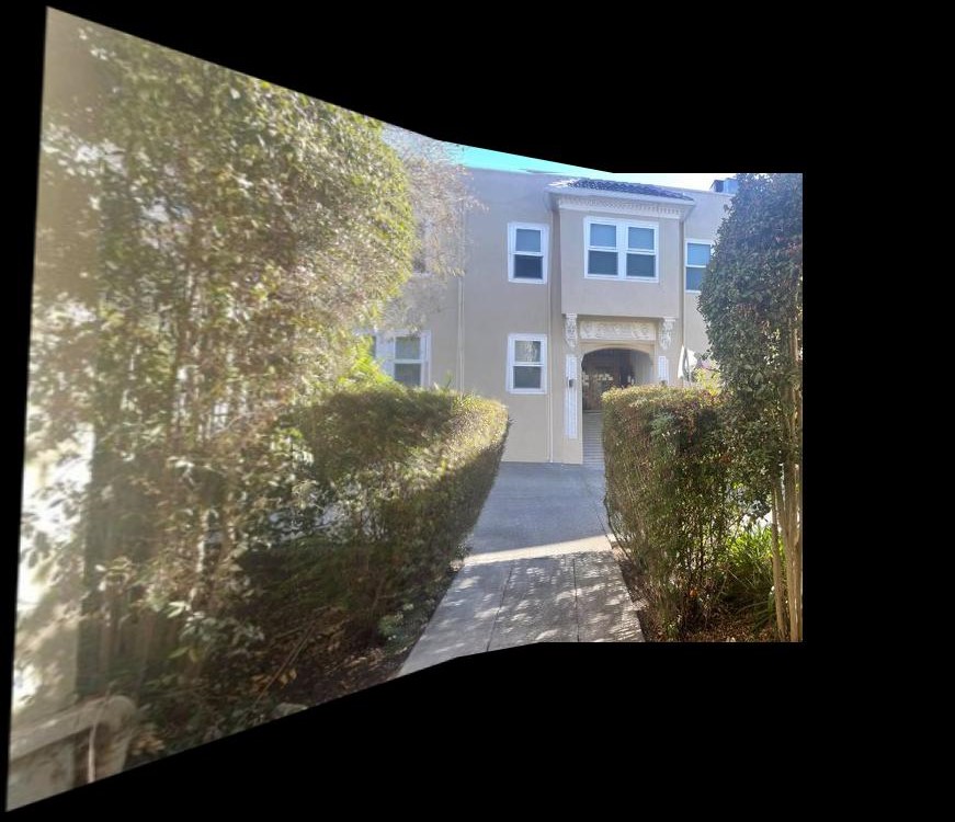
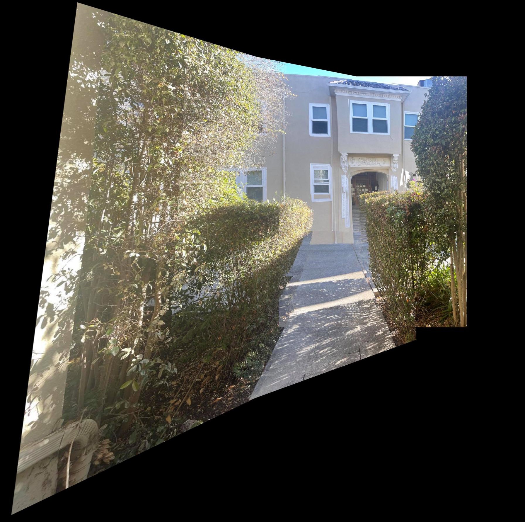
For the Front Lawn mosaic, below are the three images that were stiched together:
For the Haas mosaic, below are the three images that were stiched together:
The coolest thing I learned from this project is how to do different calculations in order to align the warped photos, create the correct canvas size, and tranform pixels from the original image. It was definitely challenging for me to picture how the images would transform and determine what mathematrical operations were needed to result in the correct transformation on the merged image canvas. Some of my image resolutions were also very large, which made stitching more challenging, and I also had to resize my images.
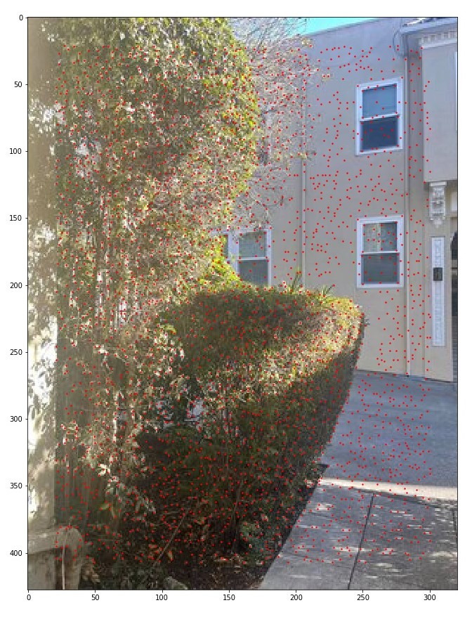
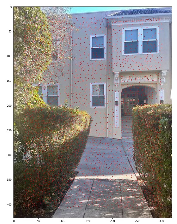
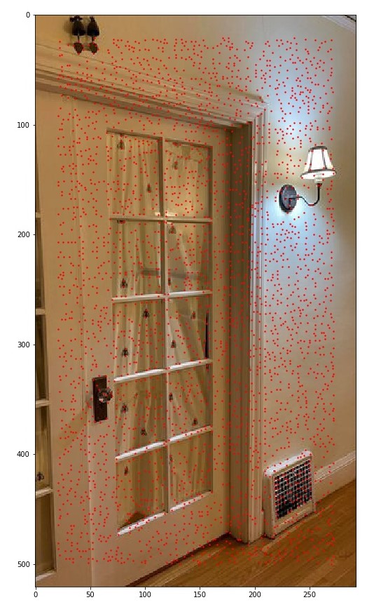
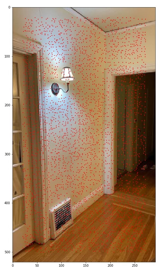
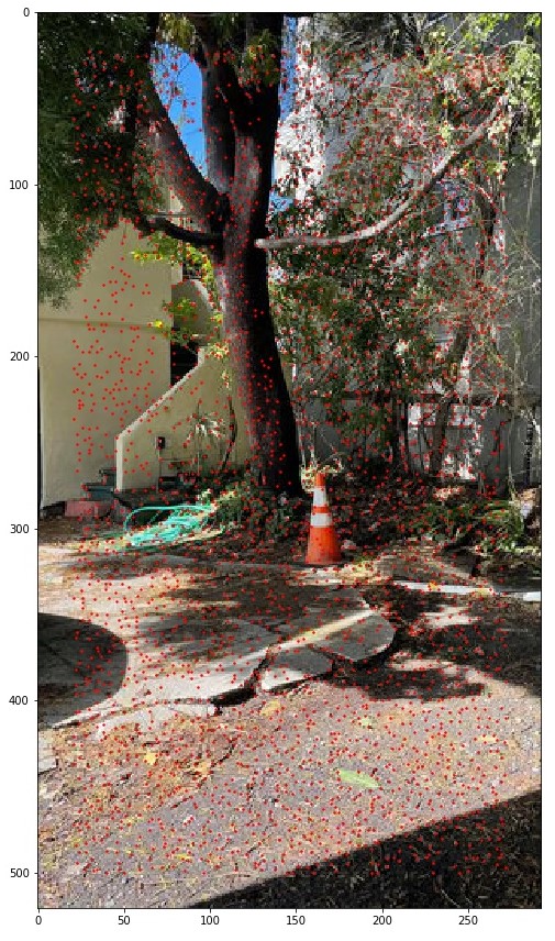
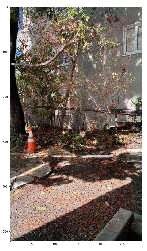
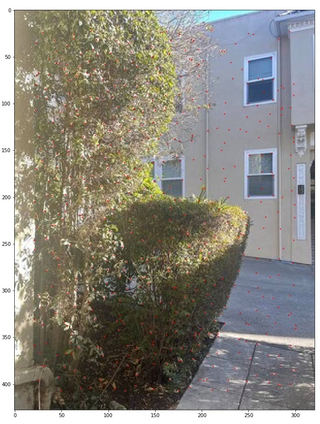
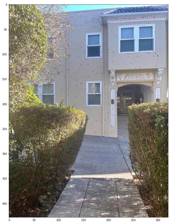
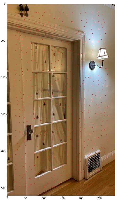
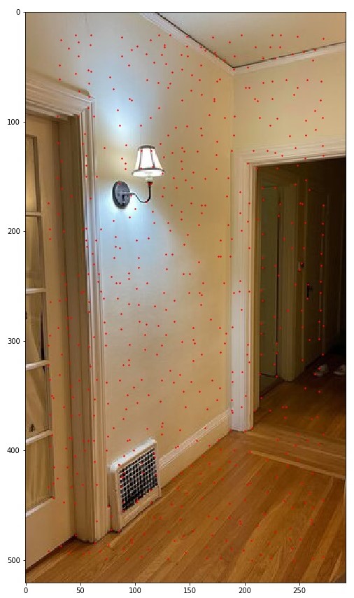
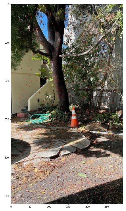
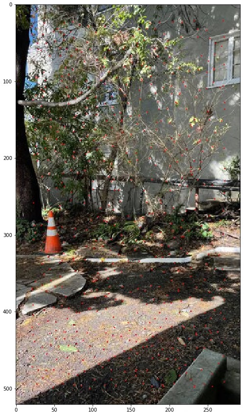
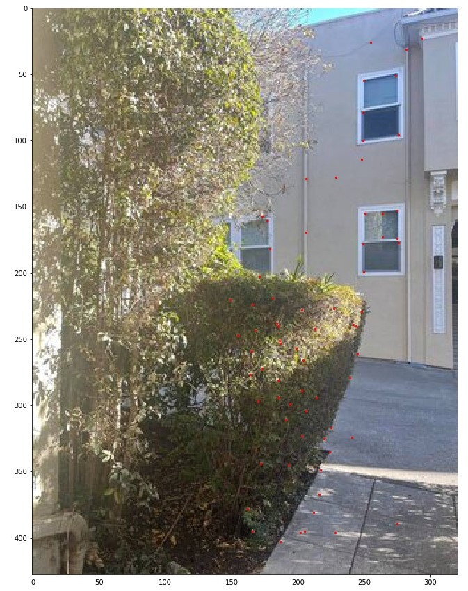
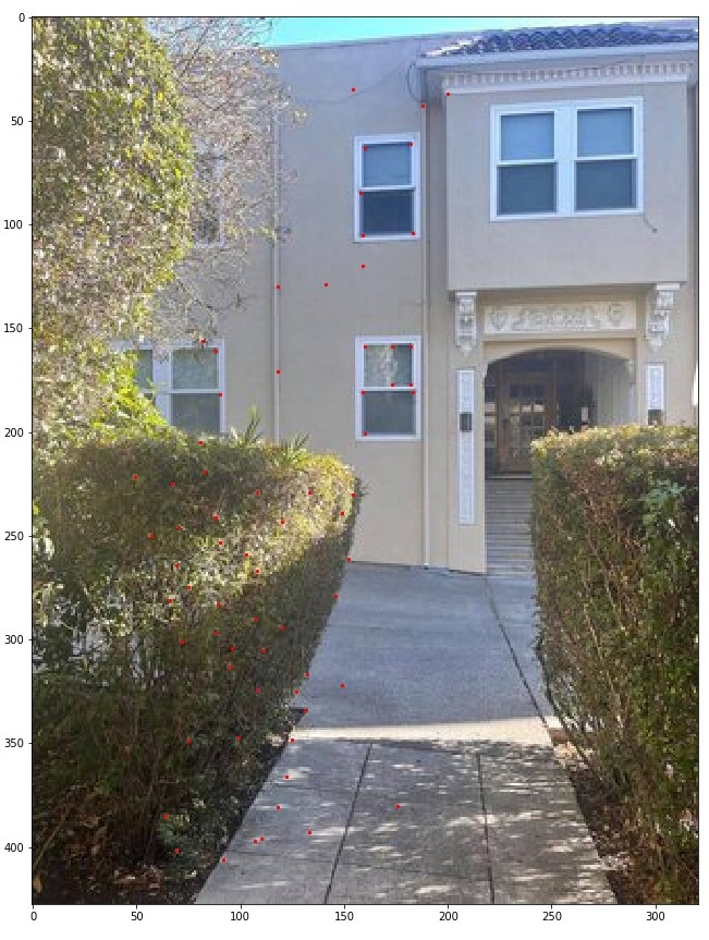
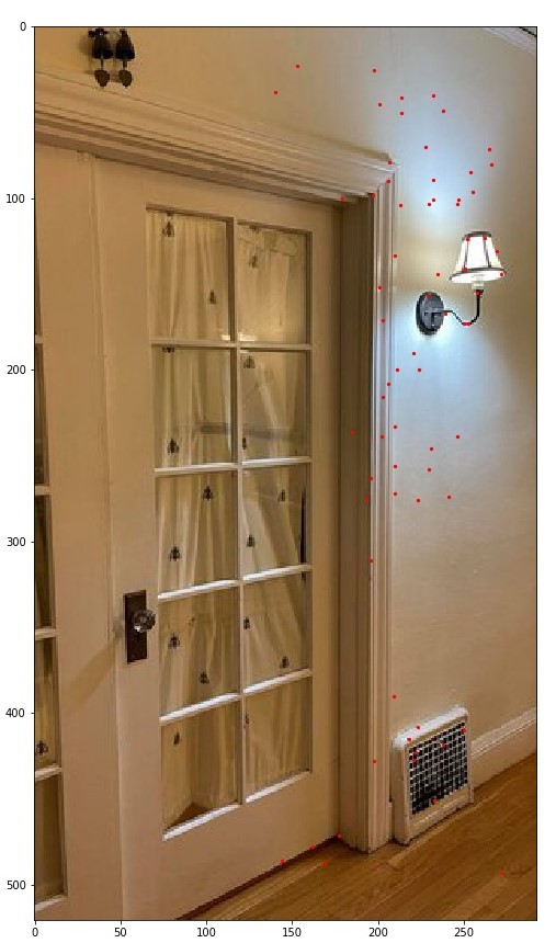
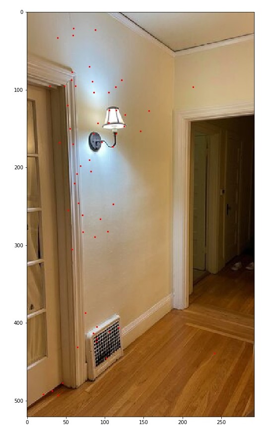
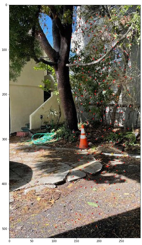
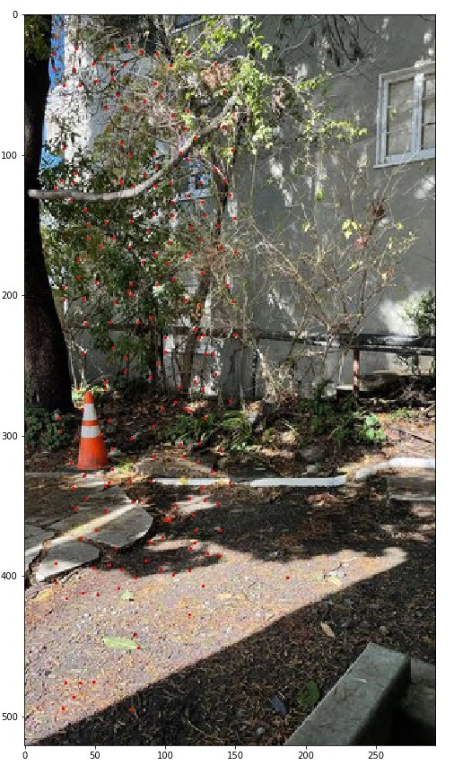
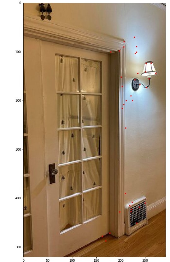
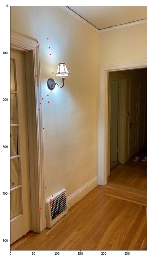
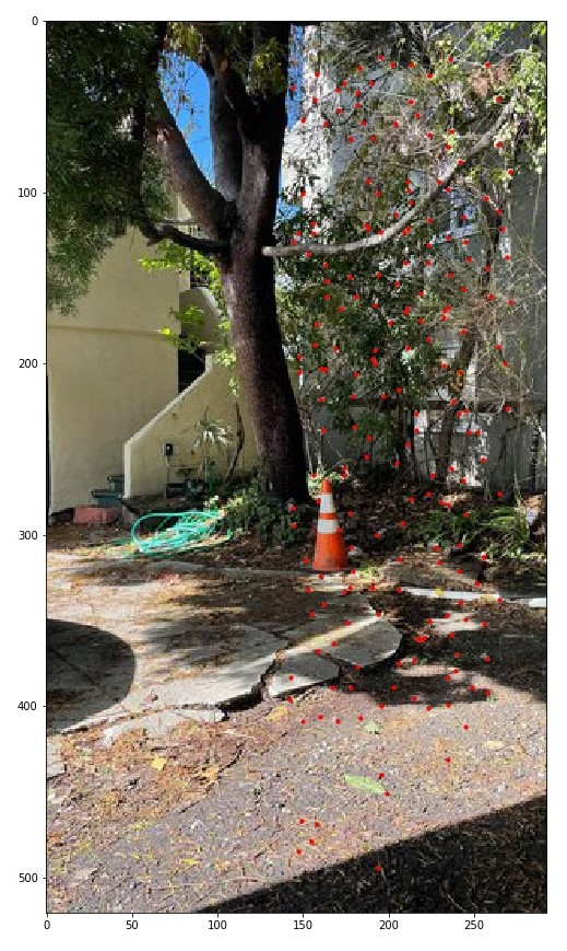
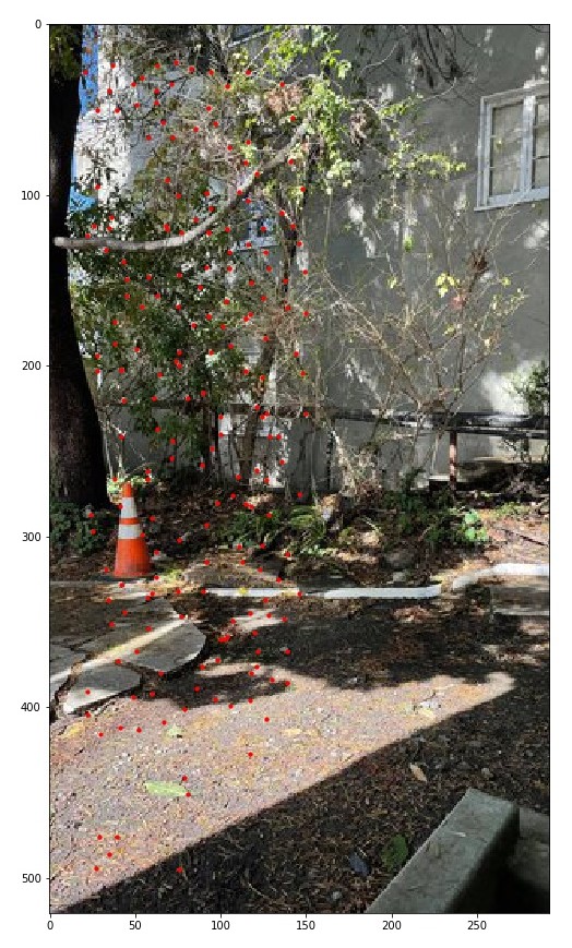
Using the starter code given, I generated Harris points for both images. The original images had too high resolutions, and due to the computational complexity of the ANMS algorithm later on, I resized my images to be around 300*500 pixels. Below are visualiztions of the Harris points on several images.
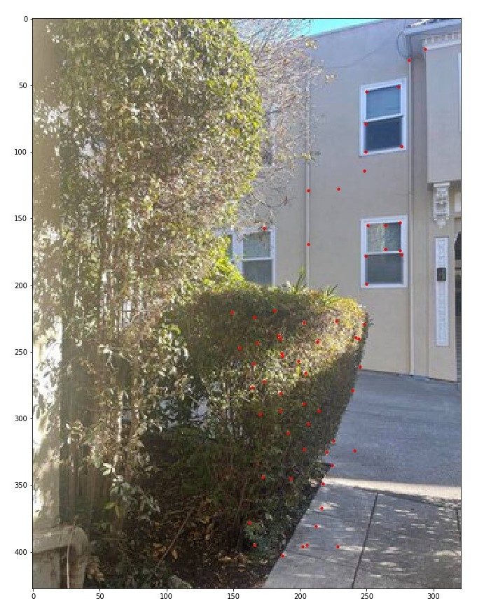
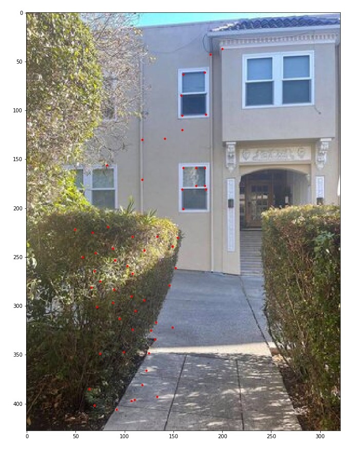
I implemented the algorithm by iterating over all the Harris points, and for every combination with other points that H_other * 0.9 < H_pt, and find the minimum squared distance between them. Then, with the list of minimum points per point, I sorted the list in descending order and took by default the top 500. Sometimes I increased the value to 600 in order to have more points to look at during feature extraction in case the end feature extraction results were sparse.
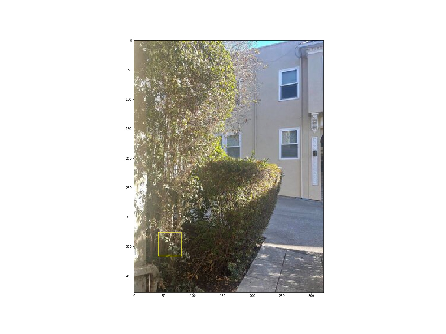
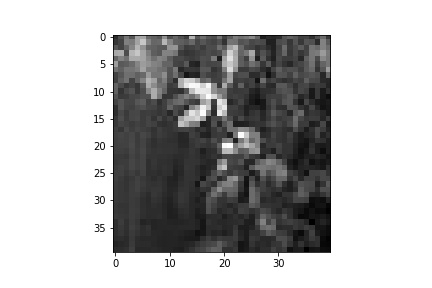
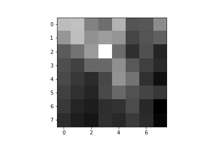
To extract features, for every point in the ANMS output, take a 40x40 sample around that point, then downsample to a 8x8 patch using sk.transform.rescale. Store this patch as a 64 length vector. To match features, after getting the feature from img1 and im2, we use Lowe's thresholding to only add features where the best distance / second best distance/error between the feature from img1 and feature from img2 is less than the given threshold. I selected 0.3 based on the paper. This method is intuitive because we are looking for features that are very similar and clearly different from the next most similar feature. Below are the results of feature extraction and the matched feature points.
For the RANSAC algorithem, at each iteration, take a random sample of 4 correspondence points between two images and generate a homography H. Compare the warped points of image 1 to the actual counterparts in image 2 and select the points/features that result in a squared error below the threshold. At each iteration, keep track of the size of the set of points that result in error below the threshold. At the end, return the largest set of points that have an error below the threshold. Below are exampels after 1000 iterations.
For autostitching, instead of manually selecting points, use the RANSAC selected points to stitch images together. Below are some examples using the same stitching functinos I used in 4A but now taking in RANSAC points to compute the homography transformations. Comparing the results of autostitching and manually, it is clear that autostitching resulted in better alignment and results where more even and the transformations were more exact.
The coolest thing I learned was the feature matching algorithm. I thought that the use of Lowe's thresholding was intuitive and really cool to see in action to find valuable features.