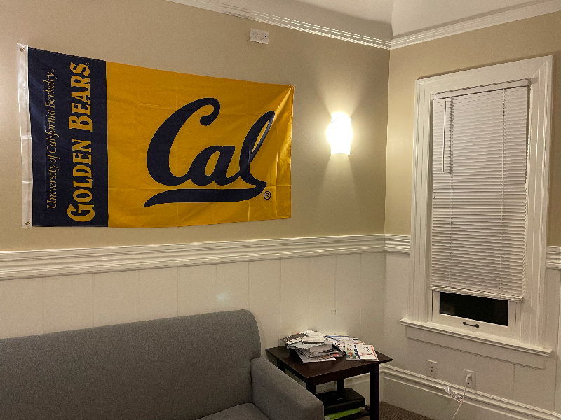
Upper Image
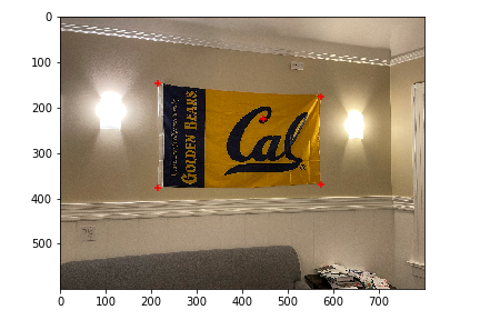
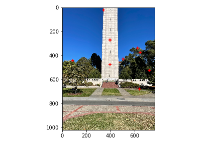
Upper Image with points
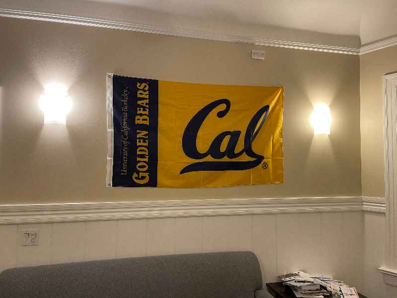
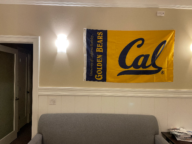
Lower Image

Lower Image with points
by: Gavin Fure
We'll be using projective warping to create image mosaics. This is pretty similar to what we've done in previous projects, but here we get to use 8 degrees of freedom in our warps!
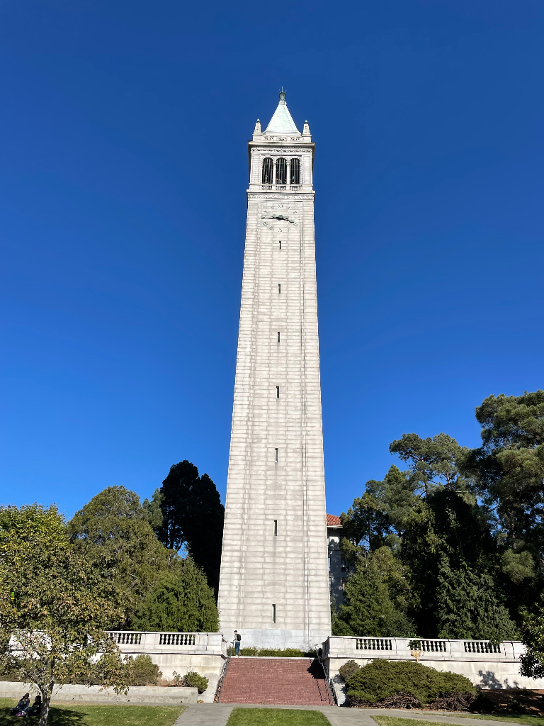
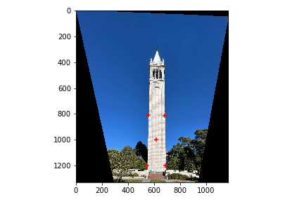
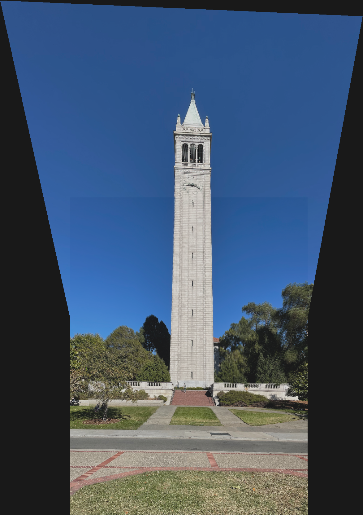
I took a few pictures of the campenile:
|
Upper Image |
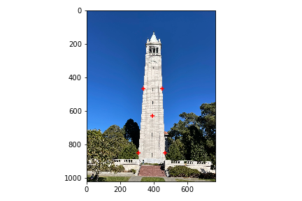
Upper Image with points |
|---|---|
|
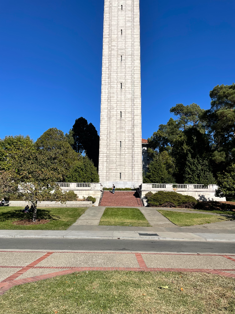
Lower Image |
Lower Image with points |
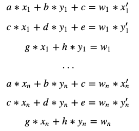
In this section we will write a function to compute a homography, a transformation matrix from one set of correspondance points to another. This homography matrix will have 8 unknowns, allowing us to perform perspective warps. The original problem formulation looks like this:
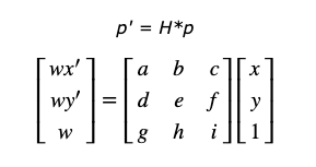
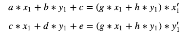
Where p is the first set of correspondances (an nx2 matrix) and p' is the second (also nx2). H is a 3x3 matrix. We can reformulate this as a system of equations, specifying for each point:
For each point, we can substiture for wi to remove it:
We can formulate this system of equations as a least-squares problem:
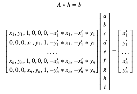
As long as we have more than 4 points, we can solve this overdetermined least squares problem!
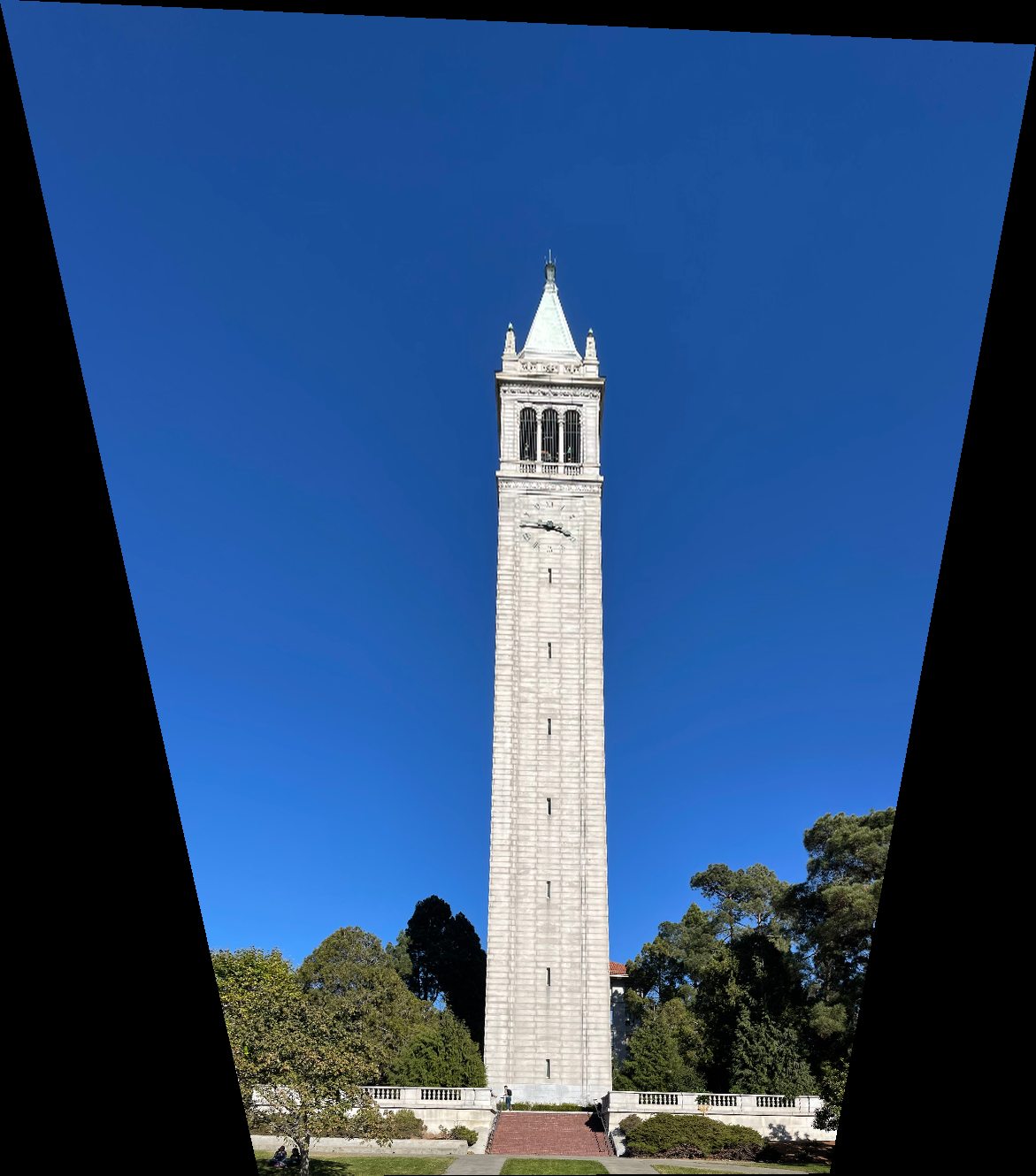
Now that we have a function that can produce a homography matrix, we can use it to transform some images. Here is the result of warping the 'upper' campenile picture to the 'lower' one's points:
Warped Upper Image |
Warped Upper Image with pts |
|---|---|
|
Lower Image |
Lower Image with points |
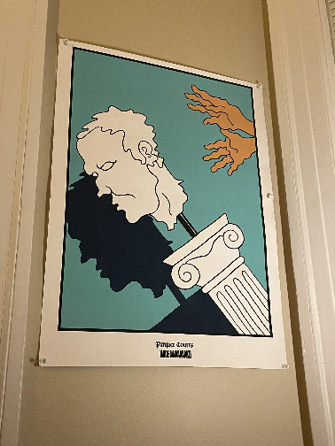
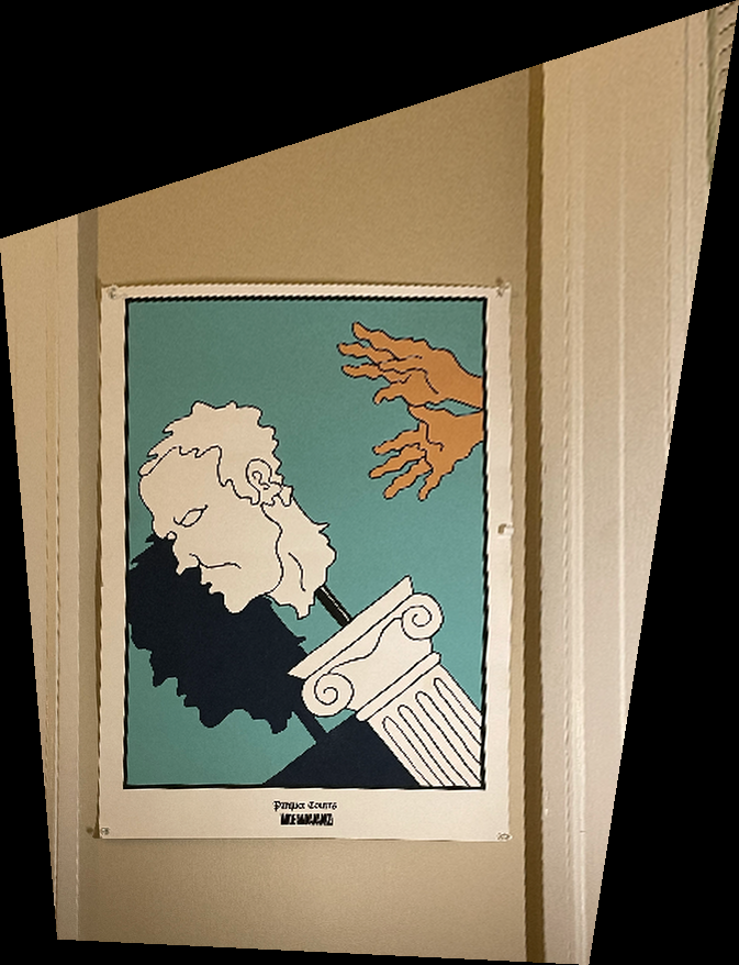
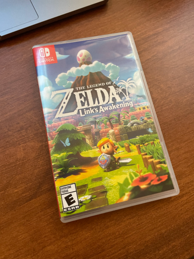
Now that our warp is working, we can warp some flat surfaces to directly face us! This is one my favorite features in phone scanner apps (like camscanner). It's really helpful, and can produce some really cool effects when applied in the right way. Here are my results:
| Original | Rectified |
|---|---|
 |
 |
 |
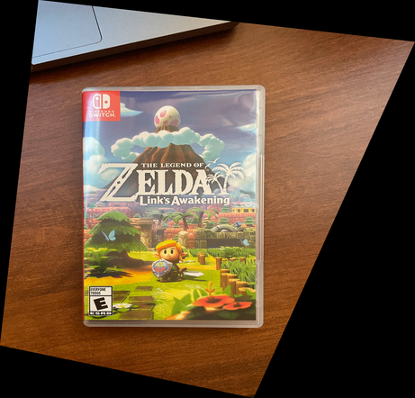 |
I used the corners of each object as correspondance points, and warped them to the corners of the image. This method was pretty quick and dirty, and doesn't preserve the original aspect ratios. That's why Link looks squished in that second warp. However, I think that this is proof our warp is working as intended!
At this point, we have everything we need to make some panoramams! We can calculate the homography matrix between the points on two images, then warp them onto the same canvase. Of course, we'll have to create a canvas that can fit all the pictures. To do this, we can send the corners of each image through its homography matrix, then use the max x and y values to create a blank canvas using np.zeros. If we have negative minimum values (which we often do!), then we can subtract the max values by the negative min values. Then, when we are warping, we can translate the results by the negative min values. This allows us to line everything up. For blending, I used a basic average mask. Each pixel value will be divided by the number of images that use that pixel. For example, if three images all include some arbitrary pixel, then the mosaic will add all of their corresponding pixel values to the output canvas. Since there are 3 of them, we divide the resulting value by 3. This is done by creating a mask (adding 1 to an empty array in the location of used pixels for each image). Then, we divide the raw mosaic by this mask.
Here are some of my results!
|
Upper Campenile |
Lower Campenile |
|---|---|
Campenile Blending Mask |
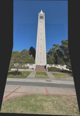
Campenile Mosaic |
This one turned out pretty good! The trees on the right are unfortunately a bit blurry, but it was windy that day so they probably moved around between pictures. There is a fairyly visible seam in the sky, because of the way I blended images. There wasn't nearly enough time for me to create a better blending option, but I think it turned out okay anyways. Let's look at another mosaic.
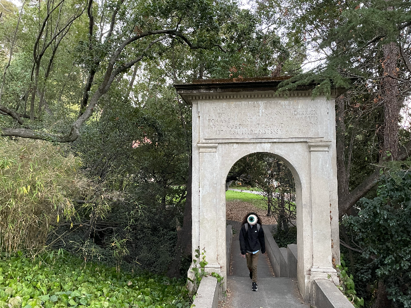
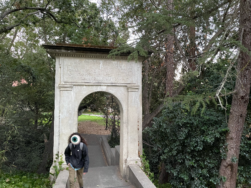
Left Gate |
Right Gate |
|---|---|
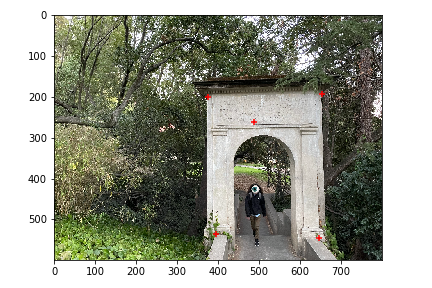
Left Gate Points |
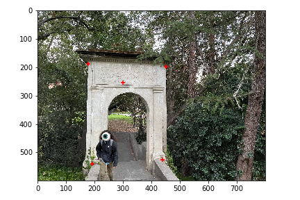
Right Gate Points |
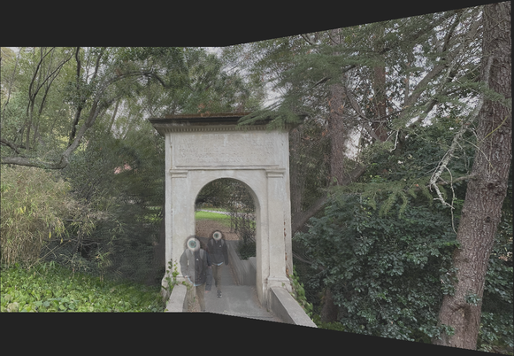
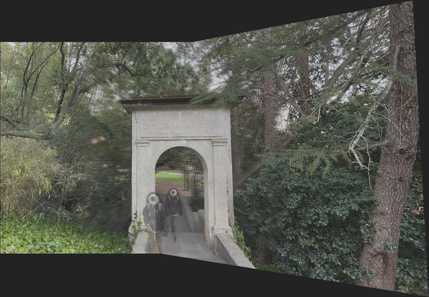
Gate Mosaic
The trees on this one are very blurry, probably also because of wind. Also a strange eyeball monster was walking through the gate while I was taking pictures, so they ended up moving. It's kind of a fun effect, they look like a ghost. The gate itself isn't as clear as it could be. This is probably due to point selection. I was only able to just click on them with my mouse (not do any sort of cross-correlation procedure around clicked points, which would definitely improve the results). This one is less successful than the others due to those factors. Let's look at one final mosaic:
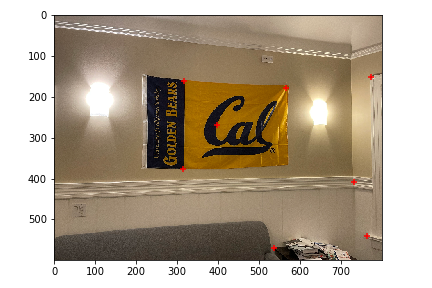
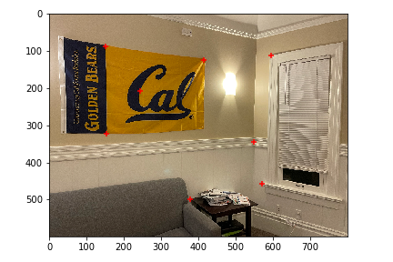
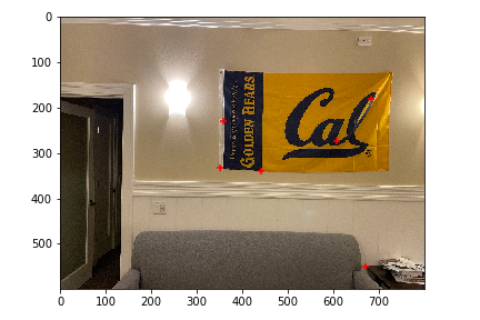
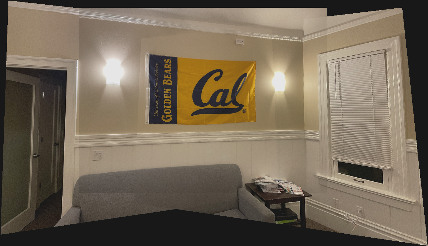
Left Flag |
Left Flag |
Right Flag |
|---|---|---|

Left Flag Points |
Center Flag Points |

Right Flag Points |
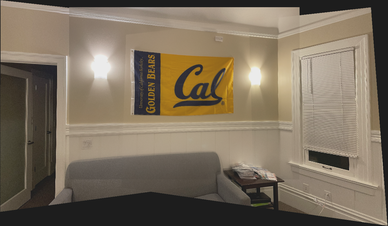
Flag Mosaic
This one turned out pretty well! It has a decent amount of edge artifacts (again due to the simplistic blending technique I am using), but besides that it looks pretty good, and it uses 3 images!!
We wrote functions to compute homographies, perspective-warp images according to those homographies, and compose warped images together to create a mosaic/panorama type image.
In this section, we will use linear algebra to automatically detect points. This will allow us to generate mosaics given only images, drastically decreasing the amount of work needed to create these mosaics. We'll be following the paper Multi-Image Matching using Multi-Scale Oriented Patches by Brown et al. to complete our project, using Harris corner detection, adaptive non-maximal suppression, and RANSAC.
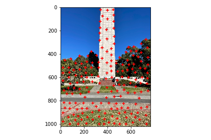
We'll be using the Harris Interest Point Detector, graciously implemented by staff as harris.py, in order to find the points that most define our image. When two images overlap (i.e. contain the same objects), the strongest points in this overlapping area should be invariant between the two pictures. We can gaurantee this with the RANSAC procedure later, but for now the Harris detector should produce similar points between the two images. It's implemented at a single scale (not multi-scale like is described in the paper). We then perform thresholding on the resulting points based on their corner strength, keeping only the strongest ones. My threshold ended up being .2, not 10 like in the paper, because the scale of corner strengths was different. The threshold reduced the number of points from 17596 to 4378 in my test image.
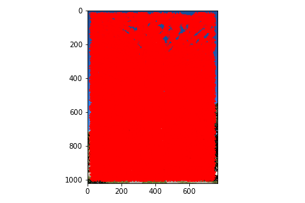
Interest Points (with no threshold) |
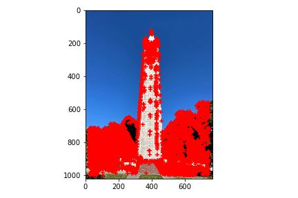
With threshold = .2 |
|---|
Adaptive non-maximal suppression (ANMS) is a process that selects the strongest points that are also well-spatially-distributed over an image. Given a set of points, we first sort them by their corner strength. We then declare the inital suppression radius to be the maximum possible distance between two points. Next, we iterate over all the points, adding the first point that is not suppressed by the suppression radius to our output. At first, our only point will be the one with the strongest corner strength, because it is first in the sorted list. This point suppresses all other points. Next, we decrease the radius by some constant scaling factor. I chose to multiply the radius by .9 after each complete iteration. We compare each point against all of the points in the output, adding only points that are not suppressed. We repeat this process until we reach the desired number of points, or until the suppression radius reaches 40 pixels (the amount required for creating a feature descriptor, which we will examine soon.) My implementation could definitely have been sped up by using the formula for the minimum suppression radius in the paper, however I wasn't quite sure how to use it. Here are my results after running my points through ANMS:
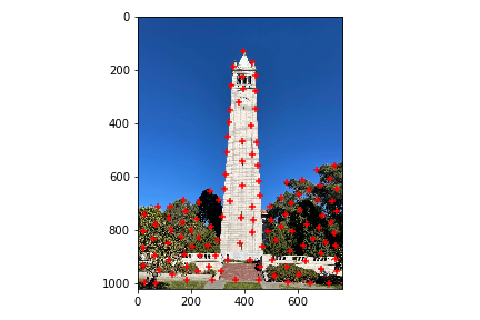
Interest Points after ANMS suppression
Interest Points after ANMS suppression
In this case (and in most cases) we reached the lower limit on suppression radius, resulting in 122 total points. As you can see, their spatial distribution is very good.
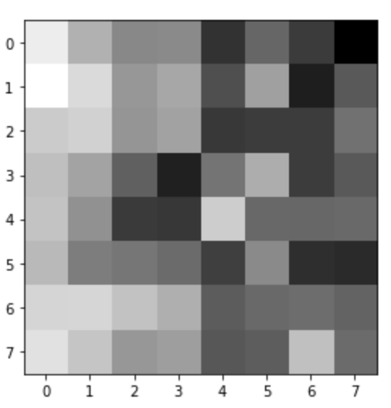
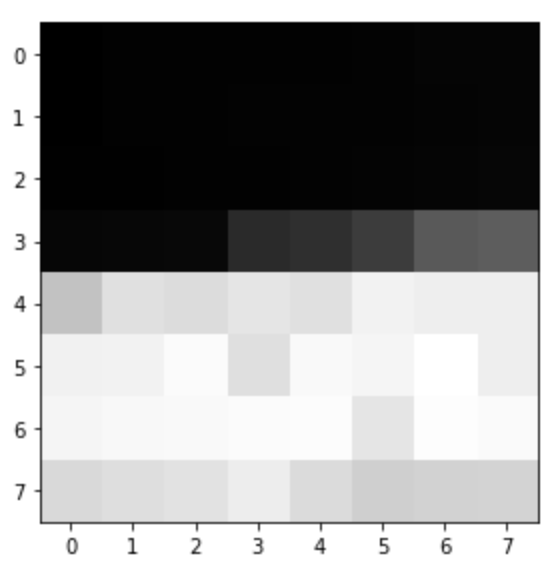
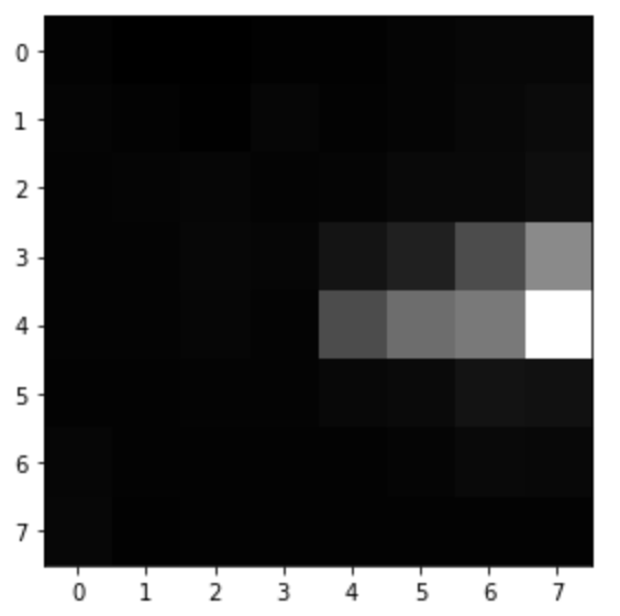
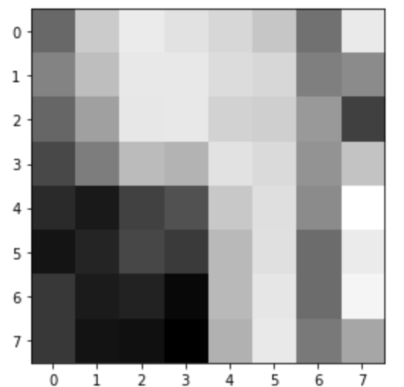
In this section, we will extract feature descriptors: little matrices that describe the areas around each point. In the next section, we'll use these feature descriptors to match similar points between two images. The process of determining feature descriptors is pretty simple: we just look at the 40x40 square around a point, then downsample it to be 8x8. Here are the results for the first five points in my test image:
|
(41, 733) |
|---|---|
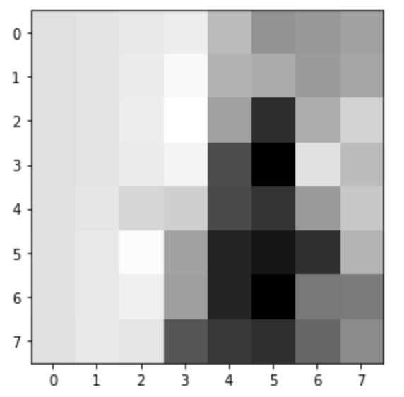
|
(336, 494) |
|
(398, 122) |
|
(504, 915) |
|
(739, 560) |
These feature descriptors appear to be pretty distinct, and they are downsampled correctly, just as intended.
To match feature descriptors together, we will calculate SSDs between each descriptor in each list. Then, for each descriptor in the first list, we will sort these ssds from best to worst (lowest to highest). Then, we will compare the ratio of the best matching descriptor's ssd to the second best's ssd. If the ratio is below a certain threshold, we will declare that point a match with its best corresponding point in the second list (the one with the lowest ssd.) This should get us a set of points that match between the two images! Of course, there is always a bit of error, but if we get the threshold right we can do pretty well! Here are my results with a threshold ratio of .5 (meaning that the best ssd has to be twice as good as the second best):

Upper campenile matched points
Lower campenile matched points
As you can see, there are some errors here, but there are enough good points to perform ransac!
RANSAC (random sample consensus) is a technique that allows us to finally get rid of as many outliers in our data set as possible. We iterate over randomly-selected groups of points, computing the best homography matrix for each with least squares. We then check this homography matrix against all of the points in our set, and count how many agree with that homography. We keep the largest set that occurs after a specified number of iterations (say 300). This is the homography that likely best represents the data set. Here are the best points from the previous point set, matched by RANSAC:

Upper campenile pts matched with RANSAC

Lower campenile pts matched with RANSAC
Alright, we have everything to compose our final function! This one is pretty special. All we need to give it is a list of images (and some parameters) and it will automatically merge two images together based on the best overlap of the two. It generates points using Harris corner detection and ANMS, matches points using feature descriptor matching and RANSAC, and then computes the homography between the set of matching points and warps them onto the same canvas. Here are my three mosaics, this time computed with automatic mosaic.
Automatic Campenile Mosaic
Next, we will look at how the algorithm performed on the gate:
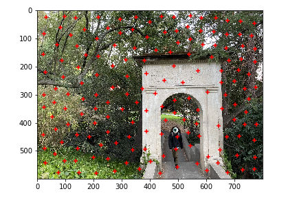
ANMS points (right side) |
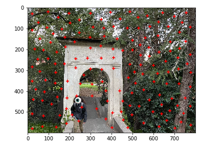
ANMS points (left side) |
|---|---|
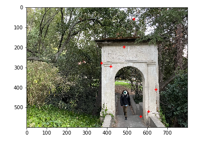
RANSAC-matched points (right side) |
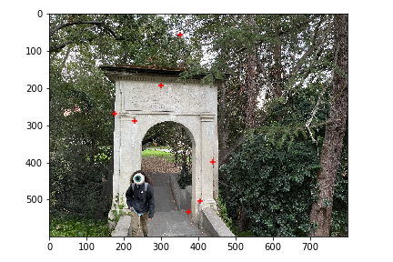
RANSAC-matched points (left side) |
Automatic Gate Mosaic
This one turned out even better than my manual mosaic! And finally, the flag:

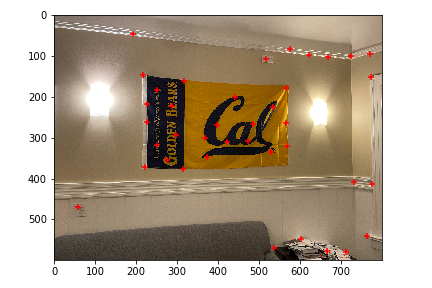
ANMS base flag points (center) |

ANMS right flag points |
|---|---|
RANSAC-matched base points (center) |
RANSAC-matched points (right side) |
ANMS base flag points 2 (center) |

ANMS left flag points |

RANSAC-matched base points 2 (center) |
RANSAC-matched left flag points |
Automatic Flag Mosaic
I've always wondered how perspective warps were performed. There's an app called CamScanner that does this kind of thing automatically, and it's always amazed me. It's so useful for scanning 2d surfaces, and it has a lot of artistic potential as well. I'm glad to know how to write a program to do that on my own!