Project 4: [Auto]Stitching Photo Mosaics
Simona Aksman
Contents
- Part 1A: Shoot the Pictures
- Part 2A: Recover Homographies
- Part 3A: Warp the Images
- Part 4A: Image Rectification
- Part 5A: Blend the images into a mosaic
- Part A Reflections
- Part 1B: Harris Point Detector
- Part 2B: Adaptive Non-Maximal Suppression
- Part 3B: Feature Descriptors
- Part 4B: Feature Matching
- Part 5B: RANSAC
- Part 6B: Creating mosaics
- Bells & Whistles
- Part B Reflections
Part 1A: Shoot the Pictures
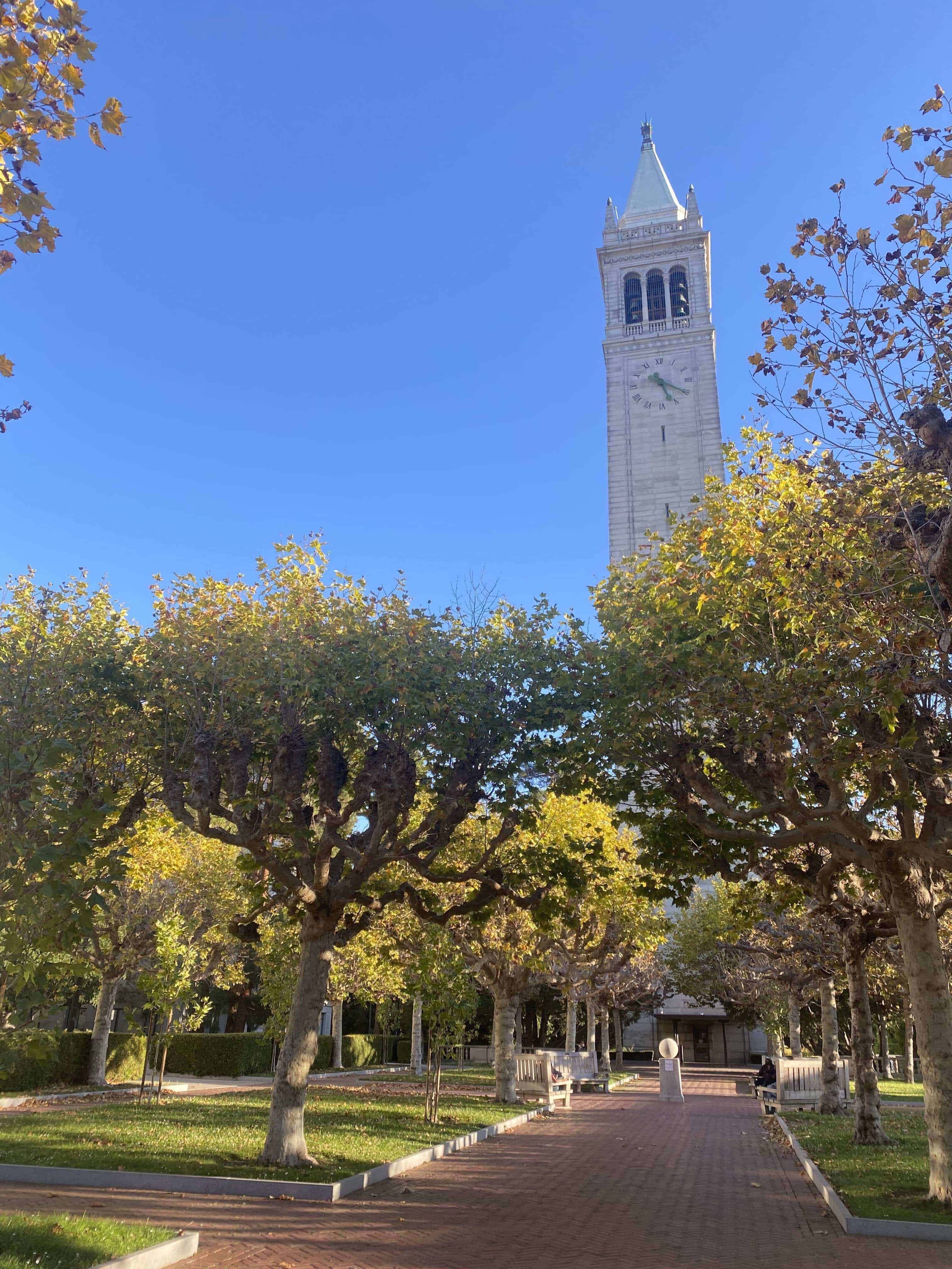
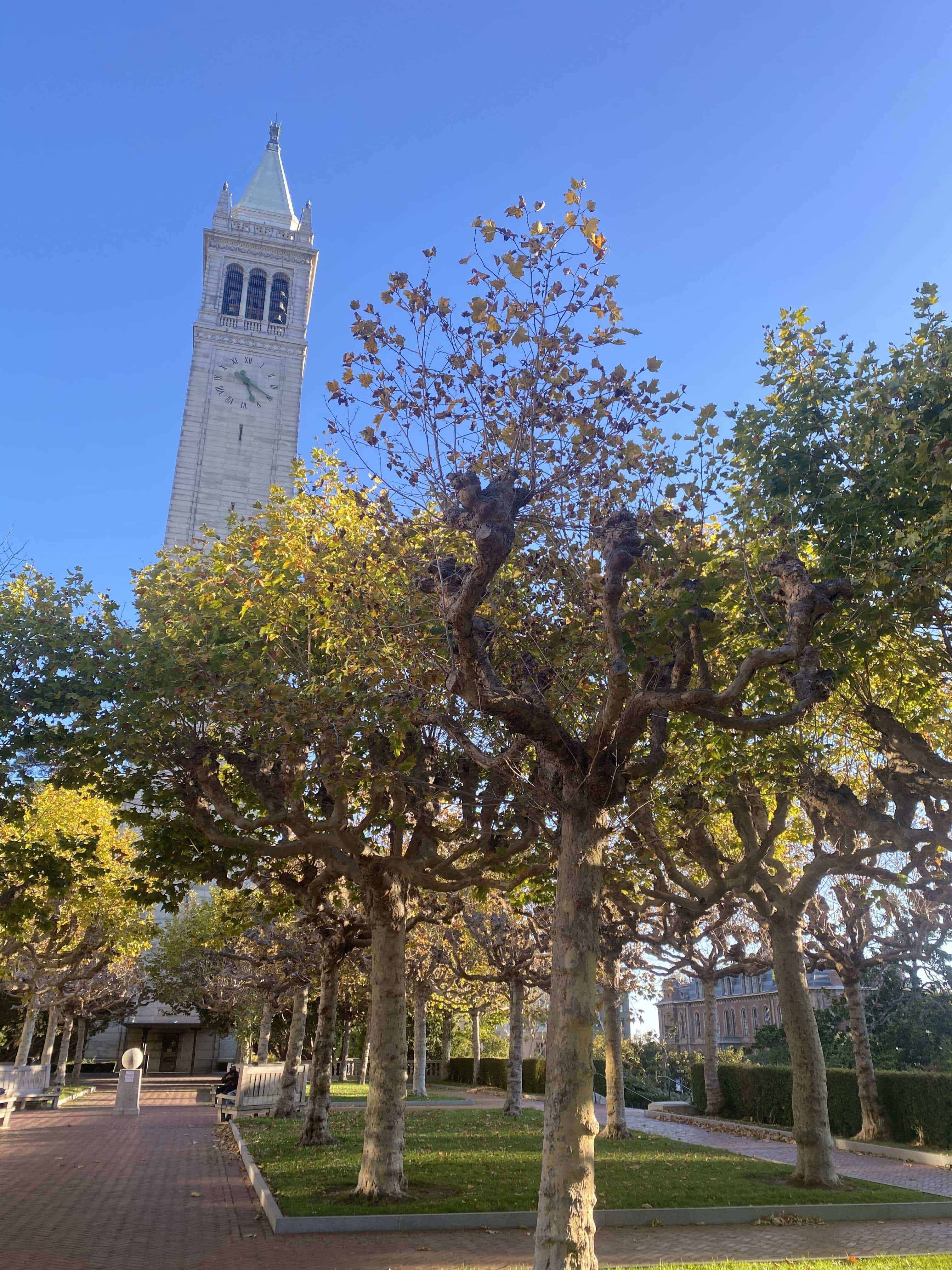
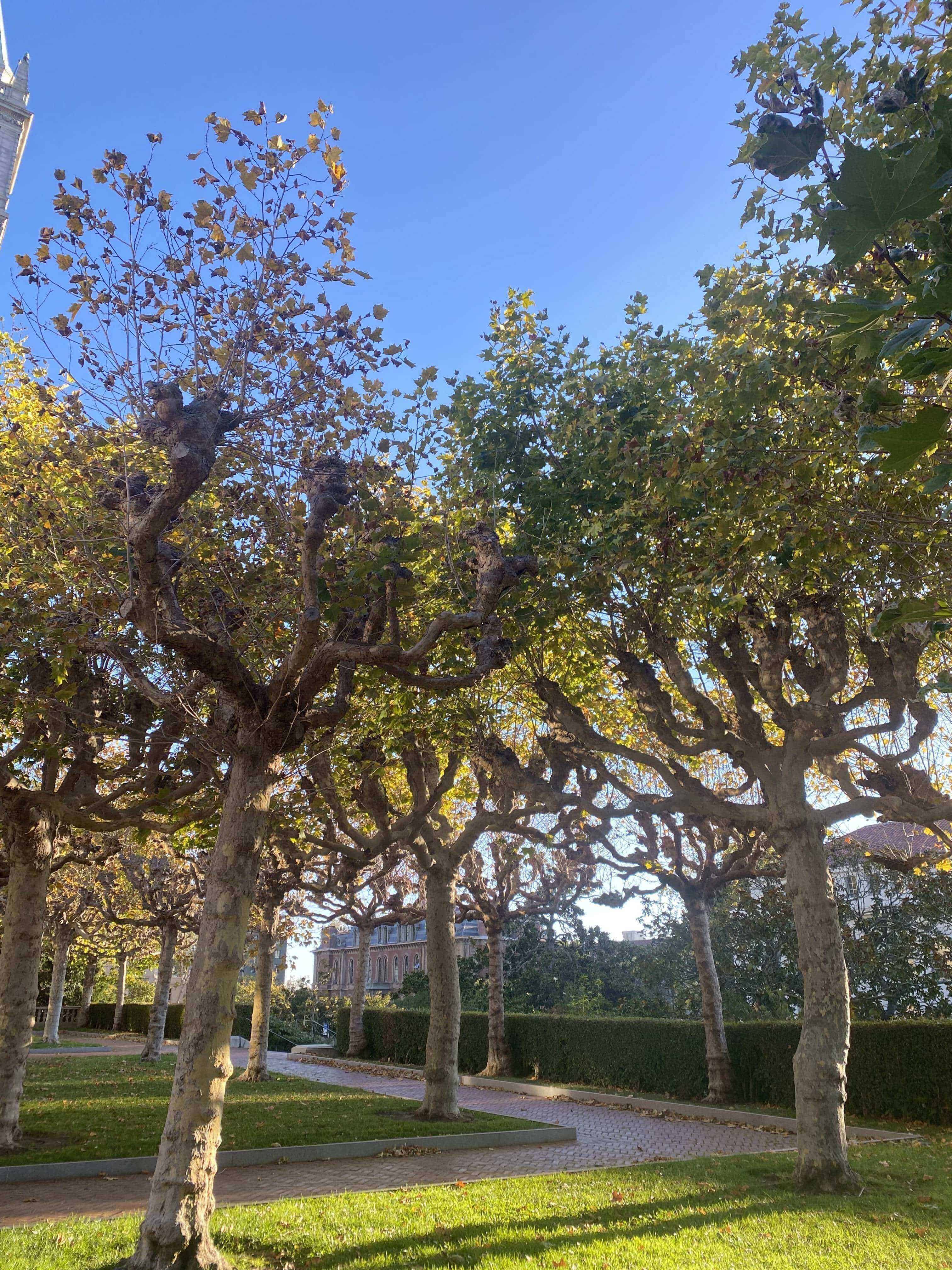
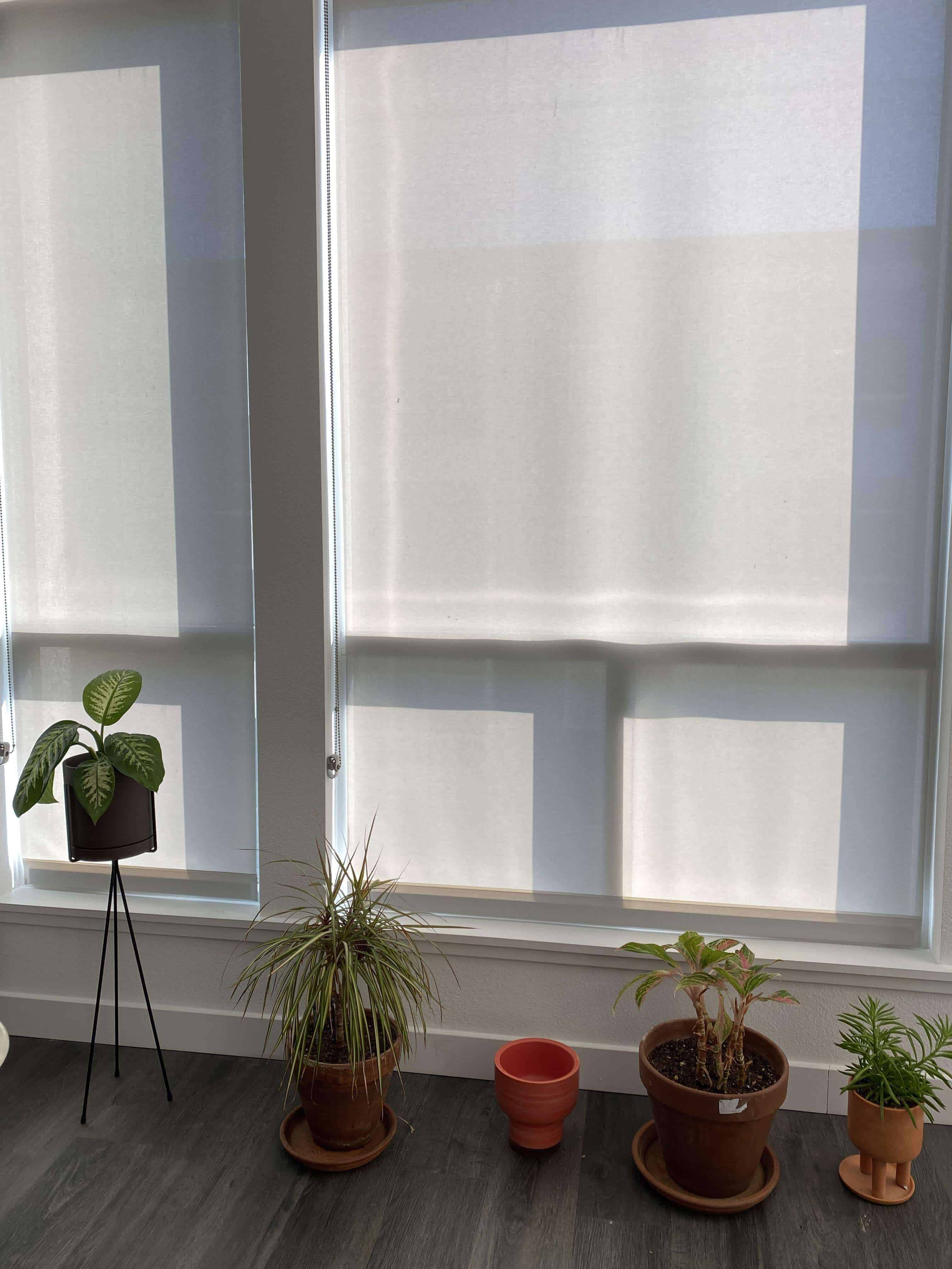
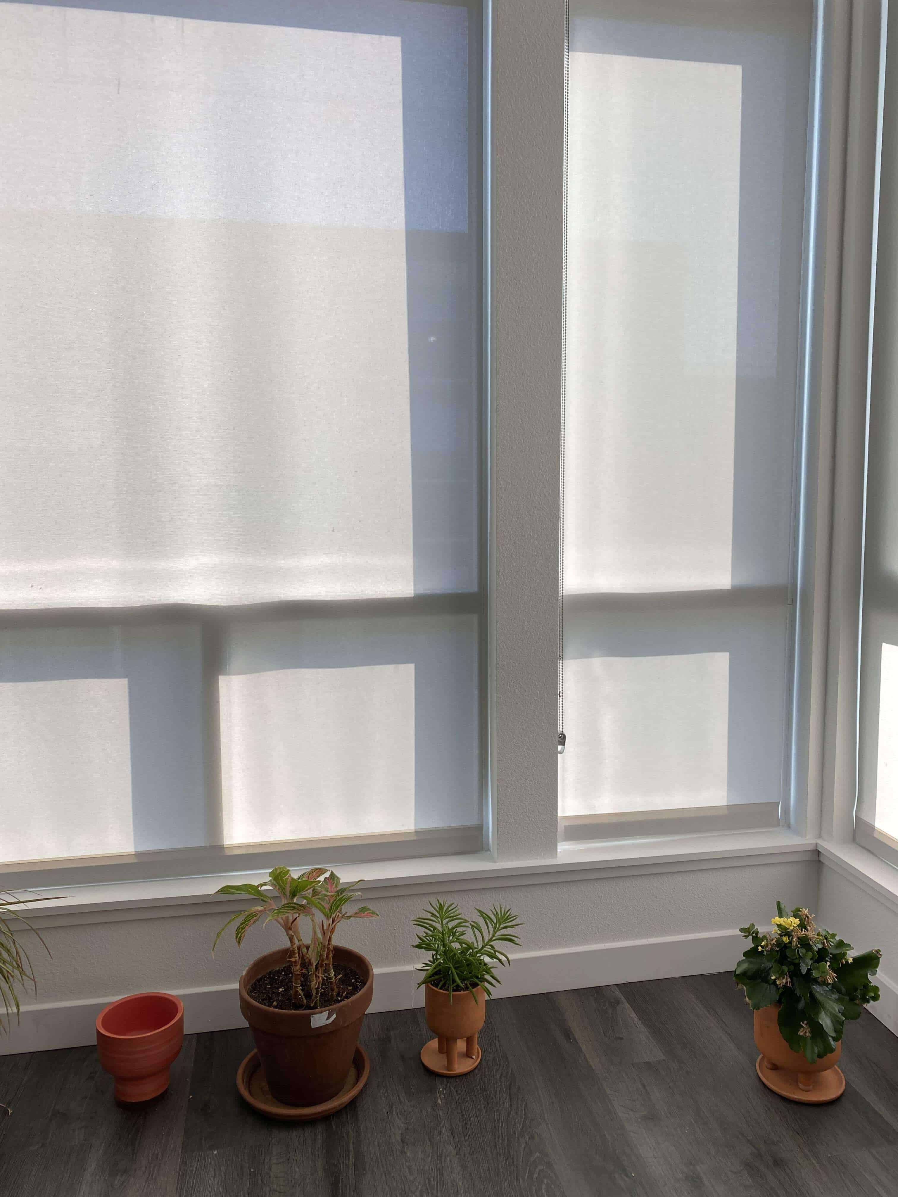
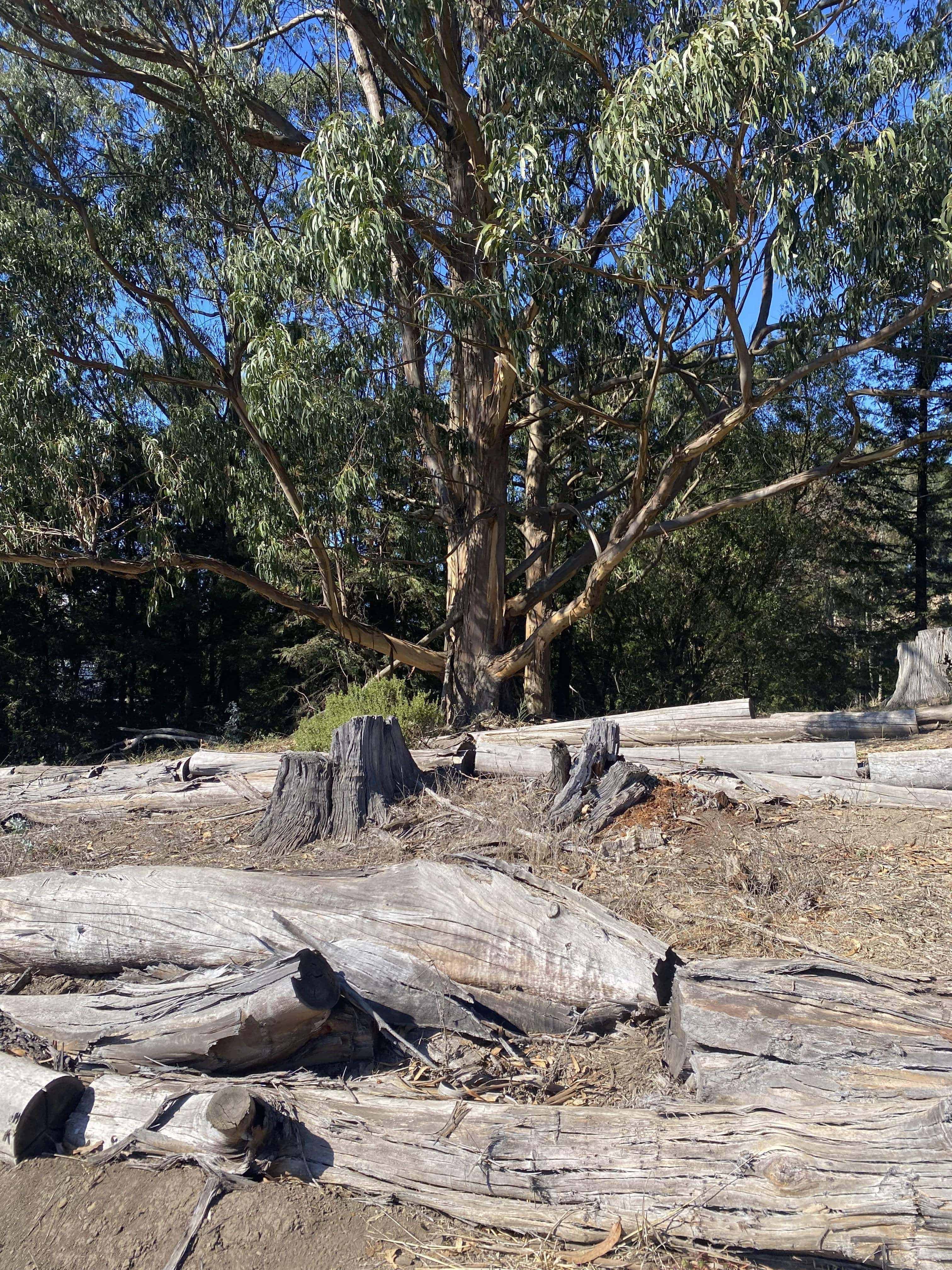
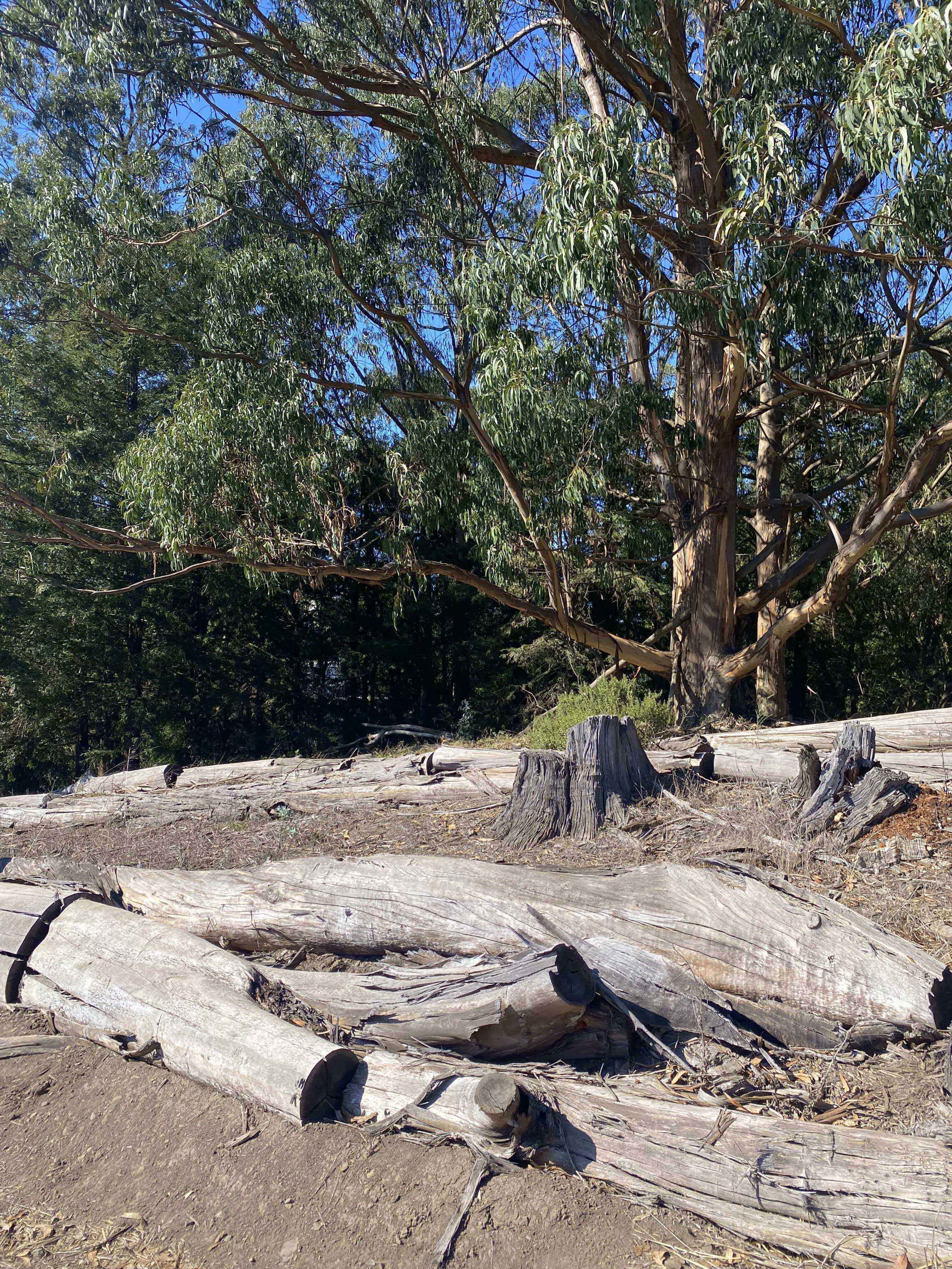
To start, I shot some indoor and outdoor photos using the approach outlined in the assignment prompt. See below for the images I selected for the project.
Part 2A: Recover Homographies
Next I worked on setting up a function that recovers a homography given at least four correspondences. At least four are needed because they produce the 8 degrees of freedom that allow you to compute a homography. However, since 4 correspondences do not always produce an accurate homography, we use an approach that supports more than 4 correspondences: least squares. To set up my correspondence to run least squares, I first expanded the homography equation outlined in class:
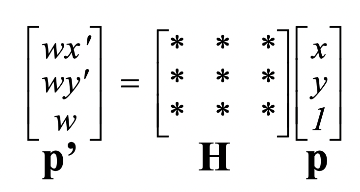
into the equation of this form:
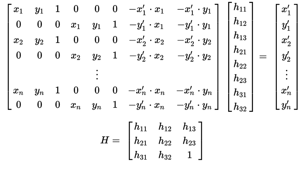
and then solved it via a least squares solver (which does this):
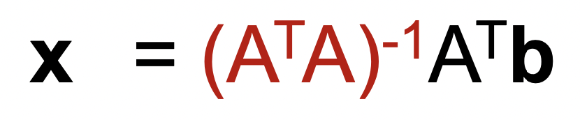
where A is is the 2n x 8 coefficient matrix, b is the 2n x 1 dependent value matrix, and x is the least-squares solution which minimizes the Euclidean distance between b and Ax.
Part 3A: Warp the Images
Then I wrote the warping function warpImage, which takes as input the image and the homography, applies inverse warping to transform the shape of the image, and then fills in the colors of the image and background using an interpolation function. The warpImage function is similar to the affine warp function I wrote for project 3, except it also handles empty pixel values, which homography transforms can generate and affine transforms do not.
Part 4A: Image Rectification
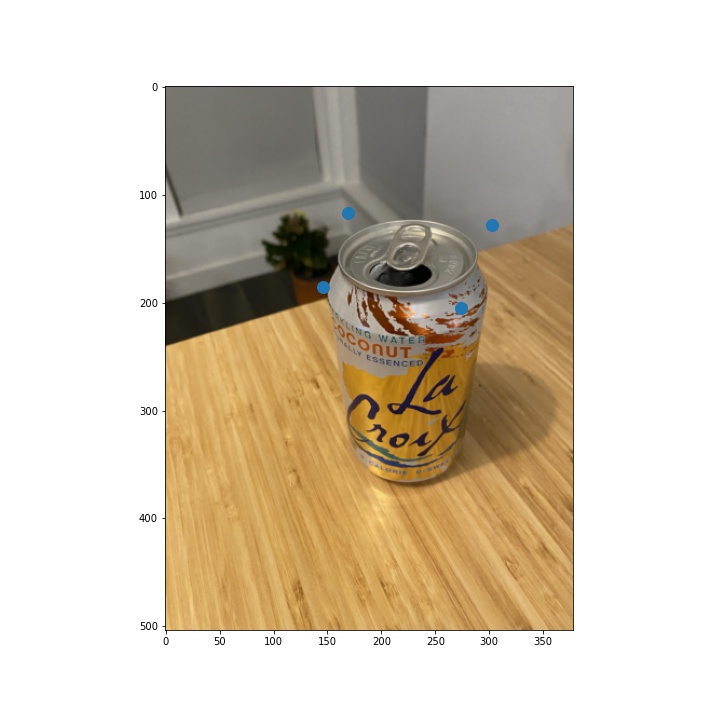
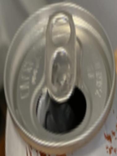
Once I wrote the warping function, I was ready to test it out. To do so, I "rectified" images: I took images which contained objects with planar surfaces and applied a homography tranformation to get an image of the frontal-parallel view of the surface. This seemed to work well overall, though some details appear blurry i.e. the small text on the book in my first example. In addition, some details were not planar in the image so they cannot be recovered i.e. the inner ridges of the LaCroix can.
Image with source mapping
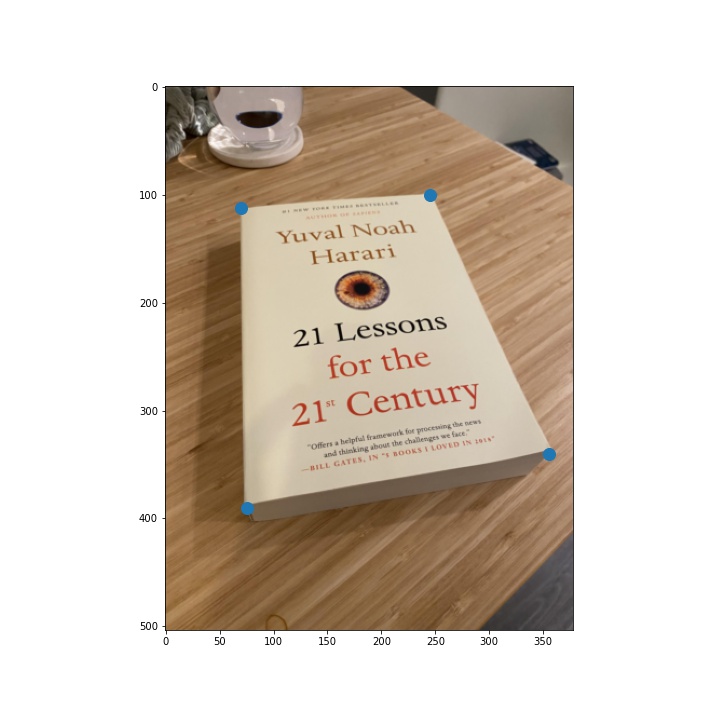
Image with destination mapping

Rectified image


Part 5A: Blend the images into a mosaic
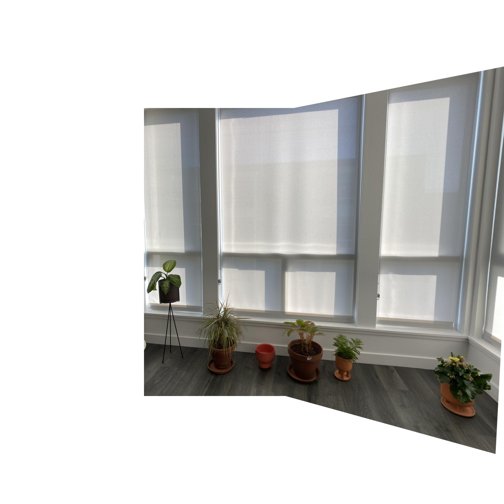
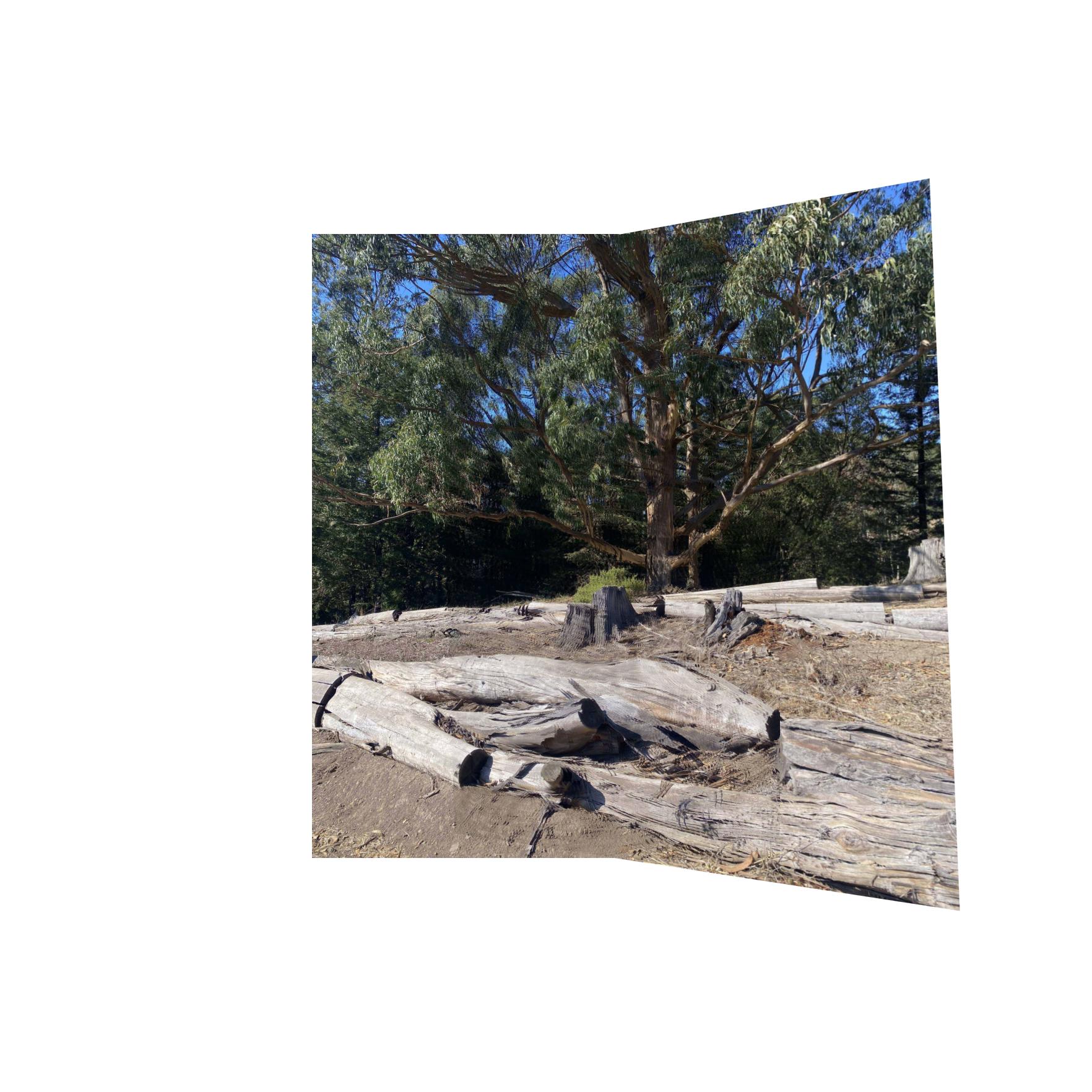
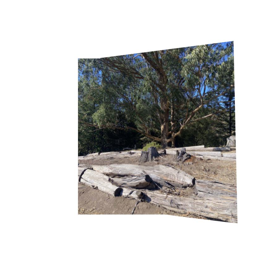
Finally, I blended the images I shot in part 1. Setting up the correspondences to ensure correct image alignment was pretty tricky, and I ended up having to do them several times to get them right. For each pair of images that I blended, I set up 10 to 20 correspondences of key features in the image depending on the image. I found that it was helped to label keypoints in a wide range of the image. When I focused my labeling efforts on just one section of an image, sometimes the other parts of the image wouldn't be well aligned.
As for how I did the blending, I found that I had decent results when I took the minimum of all of the pixel values in the images I was mosaicing (or the maximum when there's a black background). Unfortunately, there are still some traces of edge artifacts in the images after applying this blending approach. I experimented with several blending approaches (2-band Laplacian stack, alpha blending) but had trouble getting those to work well. If I have time next week, I will continue to experiment with ways to reduce the edge artifacts. In particular, I would like to try out gradient blending.
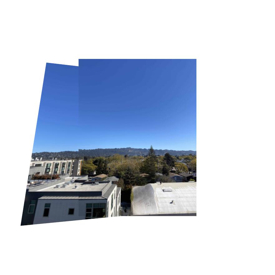
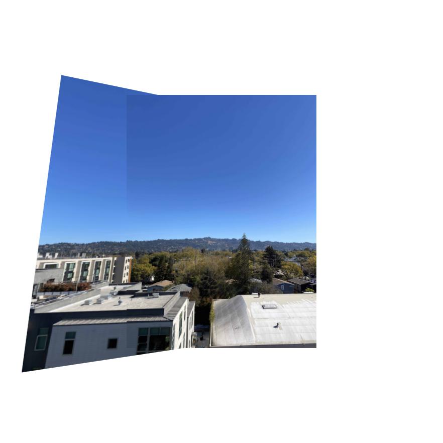
Original images
Mosaic
Original images
Mosaic
Original images
Mosaic

Part A Reflections
This part of the project was really cool because it gave me a visual intuition for how least squares estimation works. It was interesting to watch how my alignments got better as I got better at identifying keypoint candidates and piped in more of them. However, it was also quite time consuming and challenging to label the keypoints well (especially when trees were involved). I am excited for the next part of the project where we start to use methods that automate keypoint detection.
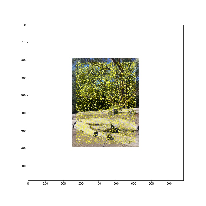
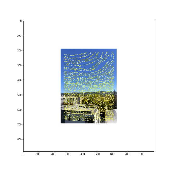
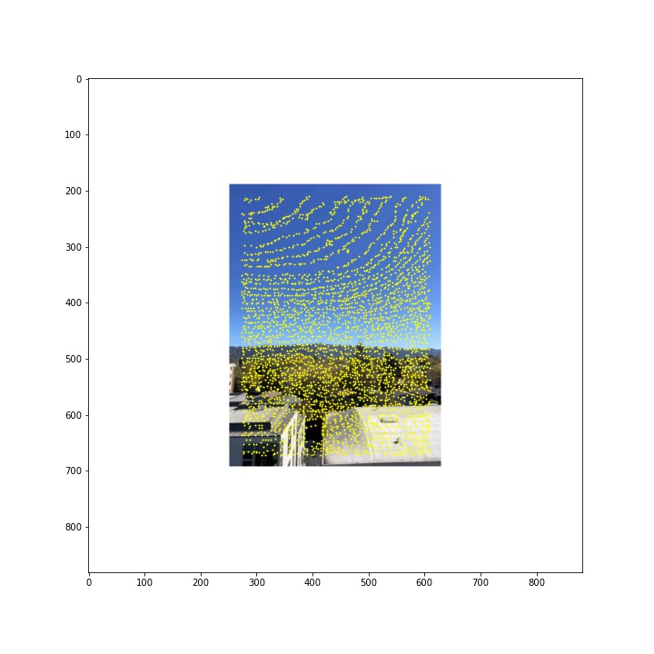
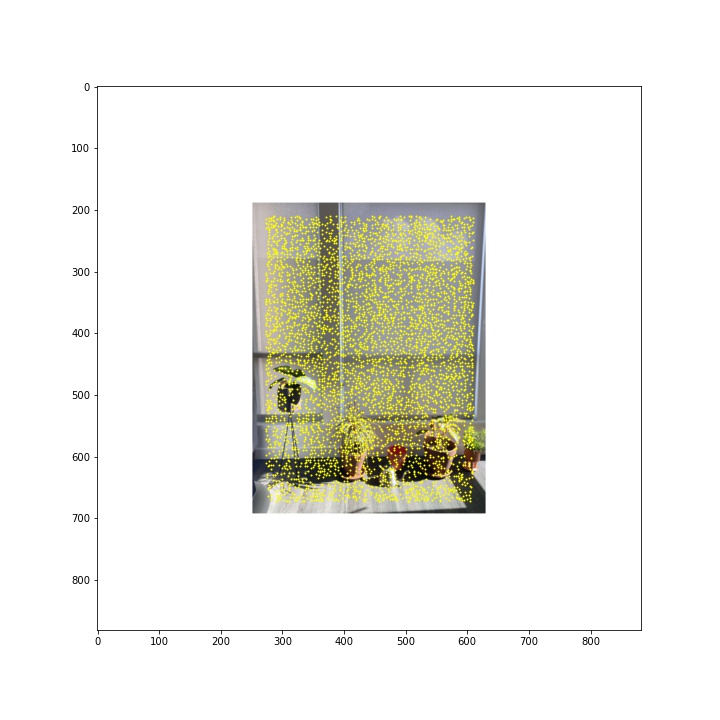
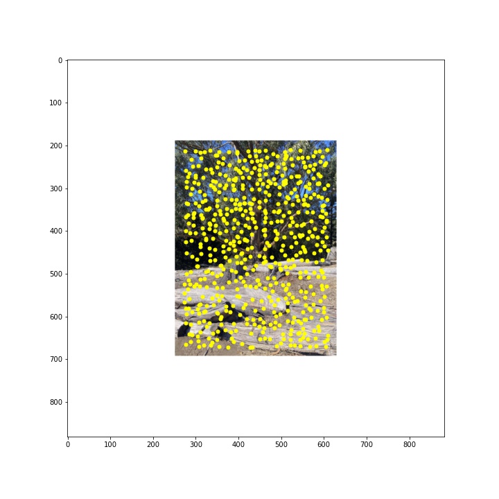
Part 1B: Harris Point Detector
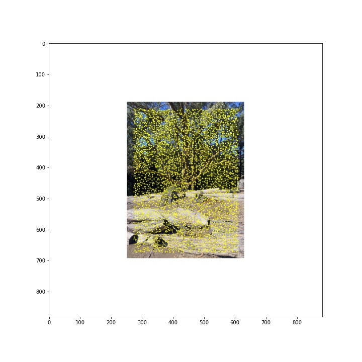
To automate keypoint detection, I started by applying a Harris Point detector, which measures the corner response at various pixel locations in an image. In my implementation, I ignore any pixels that are within 20 pixels of the image's border and set the minimum distance between peaks to 1 pixel. Harris Point detection is only a starting point, however, as it detects thousands of corners in an image. With this many corners, it is too computationally intensive to run feature matching, so next I will reduce the number of corners. See below for the Harris points detected in each of the image sets I tested with.
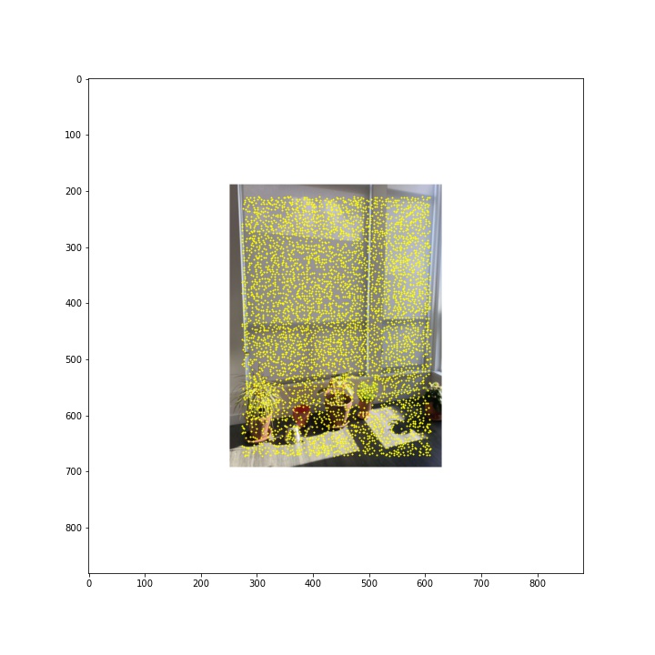
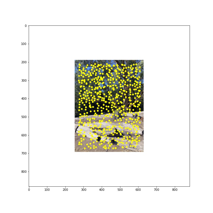
Part 2B: Adaptive Non-Maximal Suppression
Next I replicated Adaptive Non-Maximal Suppression, as described in this paper by Brown et al., to reduce the number of keypoints that need to be matched and also to ensure that the keypoints are distributed evenly over the image. This algorithm compares the Harris corner strength of points and removes points that do not have the maximum corner strength within their neighborhood to meet the objective described in the following equation:
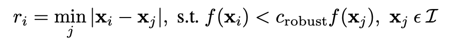
where xi and xj represent a correspondence and it's neighbor correspondence, respectively, f(xi) and f(xj) represent the Harris corner strength of each, and crobust is a multiplier that is set to ensure that neighboring point xj has higher strength than xi. Although the paper suggested that crobust should be 0.9, I found that I was able to get better results in some cases when I set crobust to be larger, such as at 1.5.
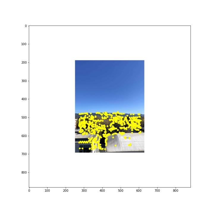
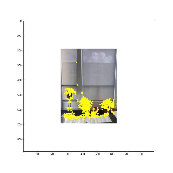
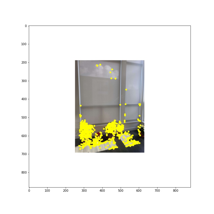
I selected 600 points from each image using this approach. See below for the correspondences chosen by this algorithm.

Part 3B: Feature Descriptors
With the smaller set of correspondences obtained in step 2, I am now ready to match correspondences between the two images. In order to do that, I extract feature descriptors for each of the correspondences using another approach described by Brown et al. in the aforementioned paper. For each correspondence point in each image, I define a 40 x 40 pixel patch equally distributed around the point's coordinates, down-sample the patch by a factor of 5 to produce an 8 x 8 patch, and then apply bias / gain normalization, producing an image patch with a mean value of 0 and standard deviation of 1. See below for some examples of feature descriptors generated through this process.


Part 4B: Feature Matching
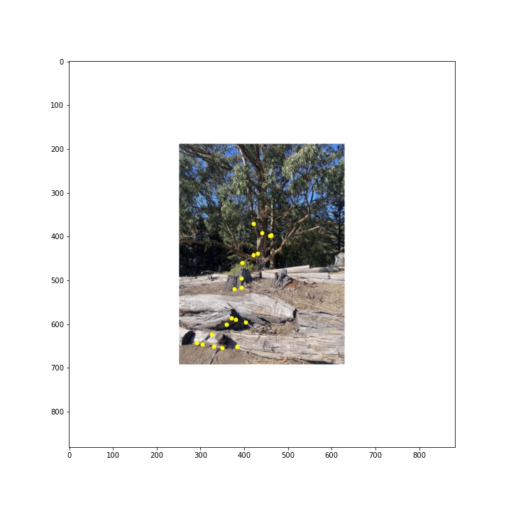
With the ANMS correspondences and feature descriptors for each correspondence point, I can now find the best match for each of the correspondences using another approach described by Brown et al. In this section, I use a nearest-neighbors (NN) algorithm to compare feature descriptors between two images using sum of square differences (SSD). Then I sort an image's matches by the SSD errors and find the top two matches that produce the lowest SSD error. These two matches are then compared using Lowe's error ratio. If the top two matches for a given image are fairly similar, the first match is unlikely to be a good match. A good threshold value for this error ratio is lower than 0.5, since that indicates that the 1st NN is more similar to the image than the 2nd NN. Applying this approach greatly reduces the set of candidate points, as shown for each example below.
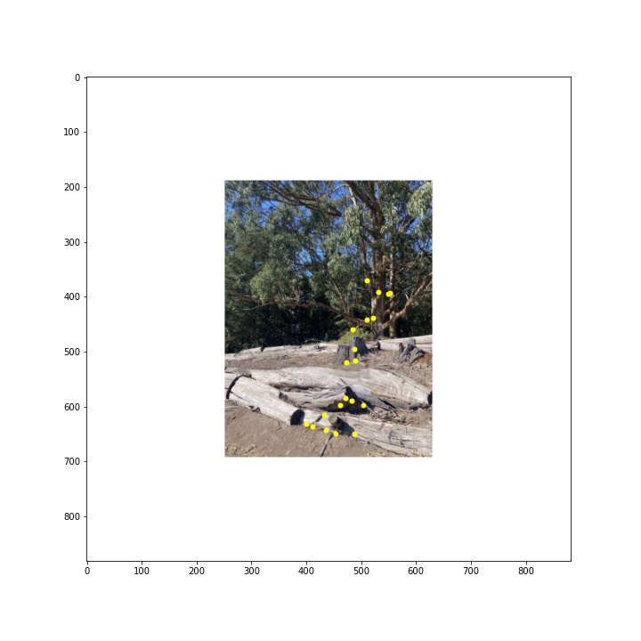
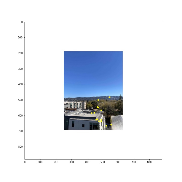

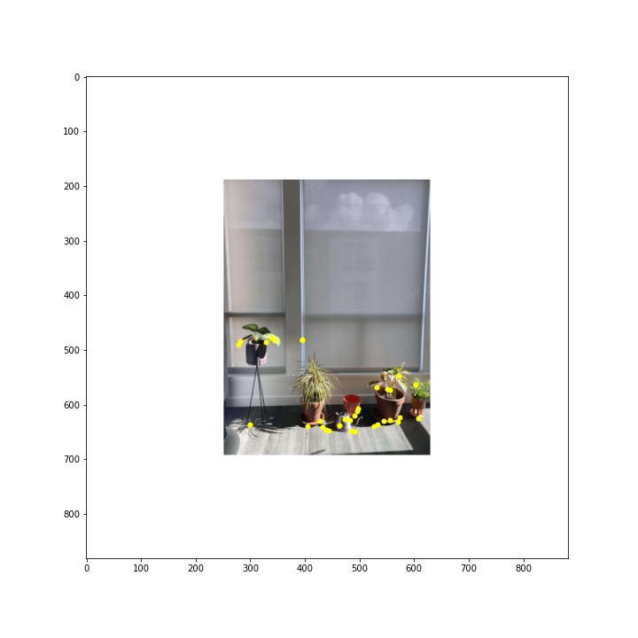
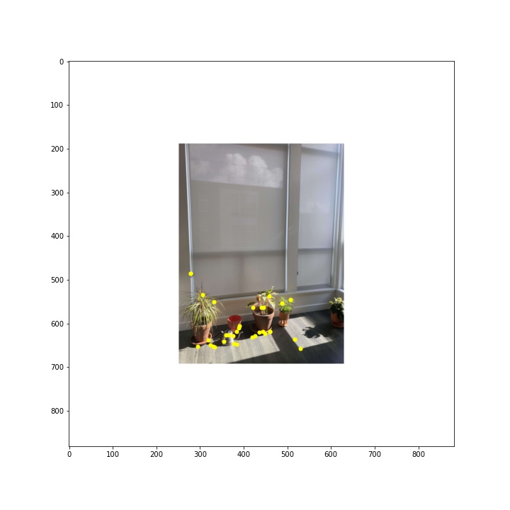
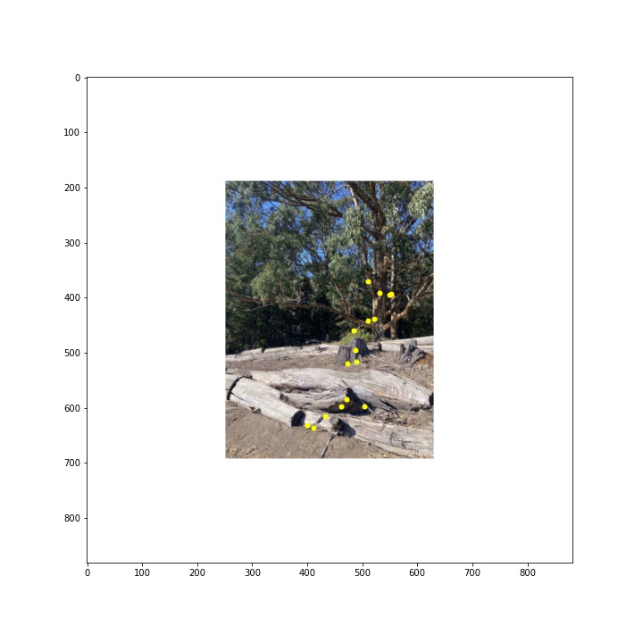
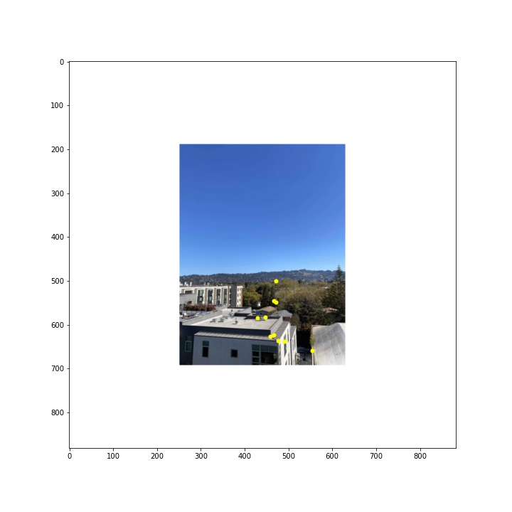
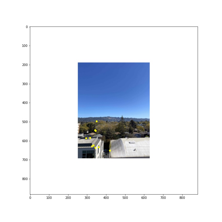
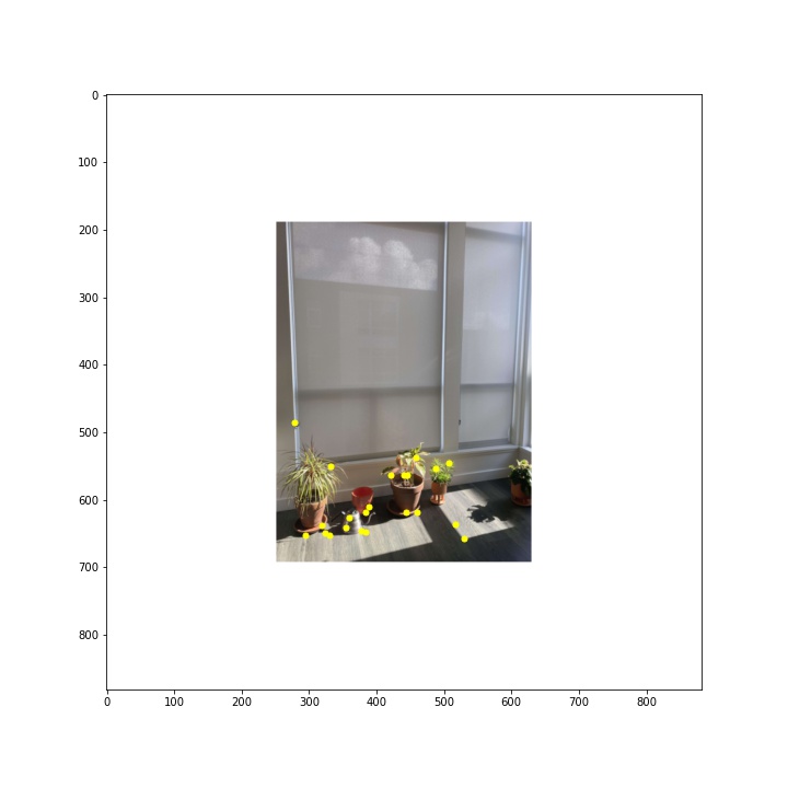
Part 5B: RANSAC
Although feature matching and using Lowe's outlier rejection rule produced decent correspondences, there are still a couple of correspondence points that are poor matches. This is a problem for computing homographies via least squares, which is sensitive to outliers. To further remove outlier points and produce a valid homography, we can use RAndom SAmple Consensus (RANSAC), an algorithm which follows the following steps:
1. Randomly sample 4 correspondence pairs from our matched correspondences
2. Compute a homography with those four correspondence pairs
3. Warp correspondence pairs using the homography computed in step 2
4. Find inliers where the homography correctly estimates the relationship between correspodence pairs. This is determined by computing the absolute difference between the pairs after applying the homography transformation and comparing it to a threshold. I found that a threshold of 2 pixels worked well.
5. Choose the homography and set of inlier points where the count of inliers from step 4 is the highest.
I reran this process many times in order to produce the matching sets of correspondences shown below. The # of iterations was another parameter I tuned for the final mosaics, and I found that for some image pairs, I only needed to run RANSAC 1000 times, but for others I had to run it 10000 times to produce a valid homography.


Part 6B: Creating mosaics
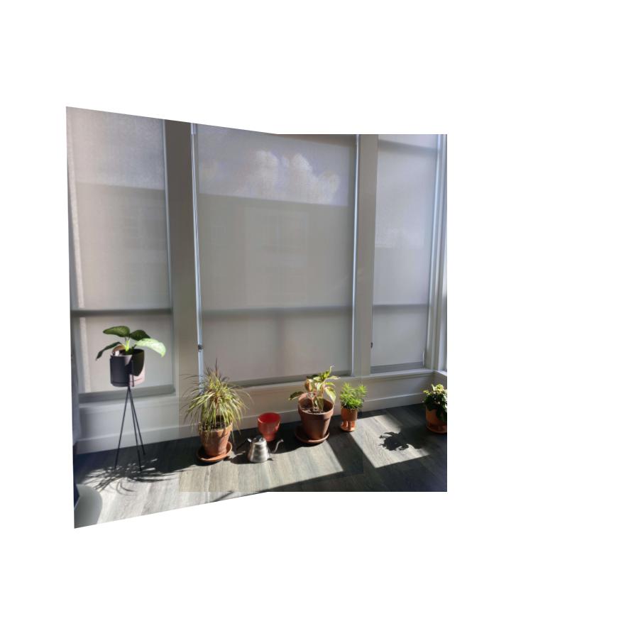
Finally, I can use the homography produced by RANSAC to warp one image to match another and produce a mosaic automatically. See below for a side-by-side comparison of the manaul mosaics I produced by labeling 10-15 correspondence points, and the automated ones produced by running the 5 steps outlined above in sequence. Note that overall, the automated approach seems to have performed as well or better than me for these examples. However, I had a few example images that it performed poorly on and I could not seem to figure out how to get it to perform well on those. I am thinking that perhaps there were too many similar textures / surfaces in those photos and the algorithm would get confused by them.Manual
Automatic
Manual
Automatic
Manual
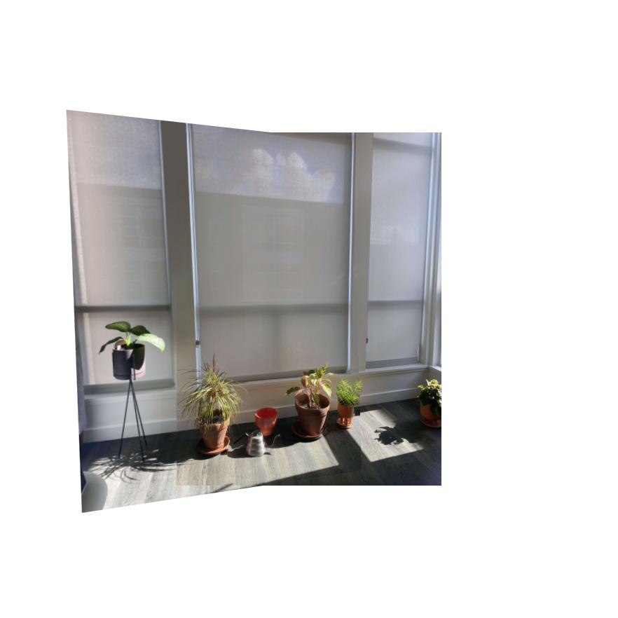
Automatic
Bells and Whistles
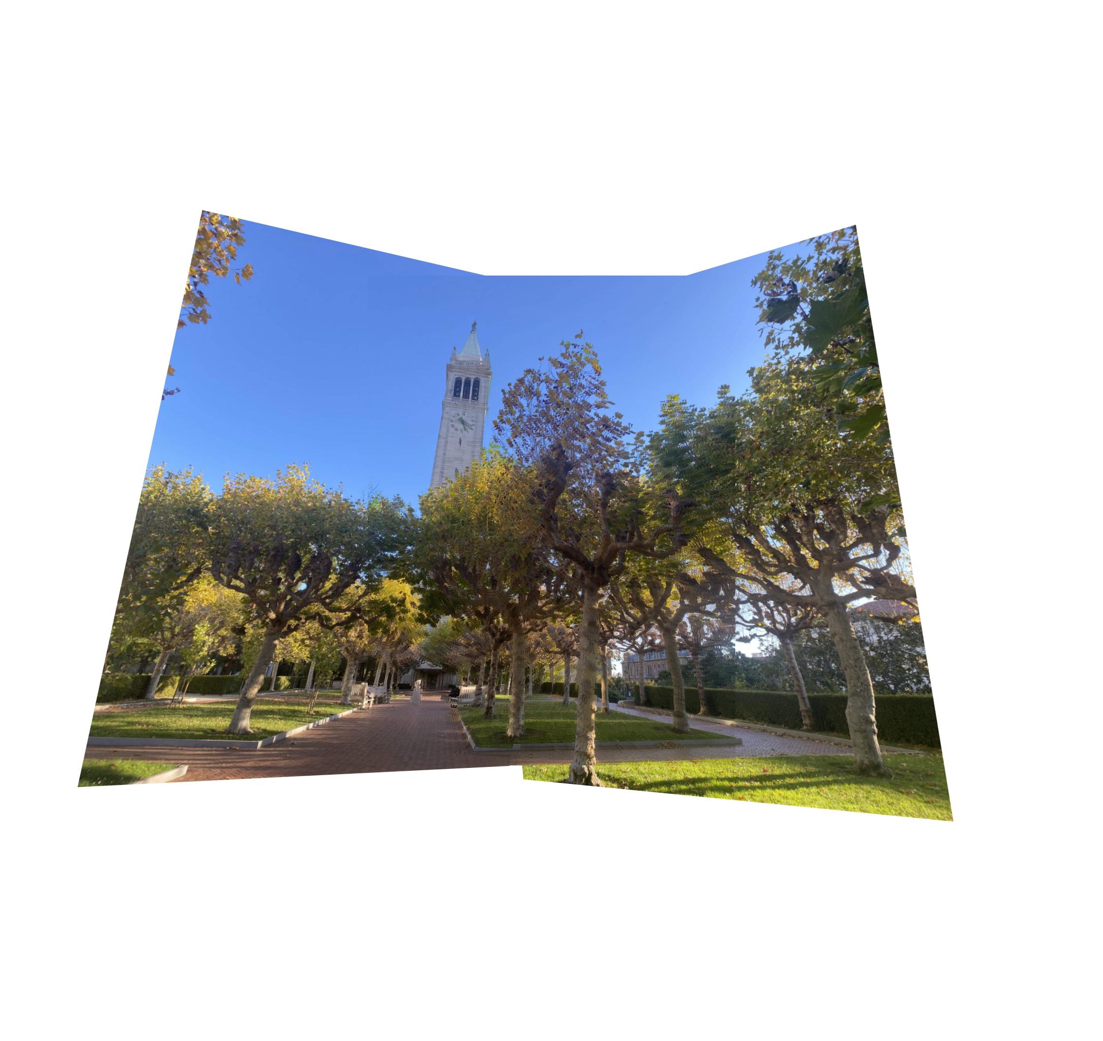
I was curious to see how a panorama would look in cylindrical coordinates. I created the following landscape panorama in cartesian coordinates:
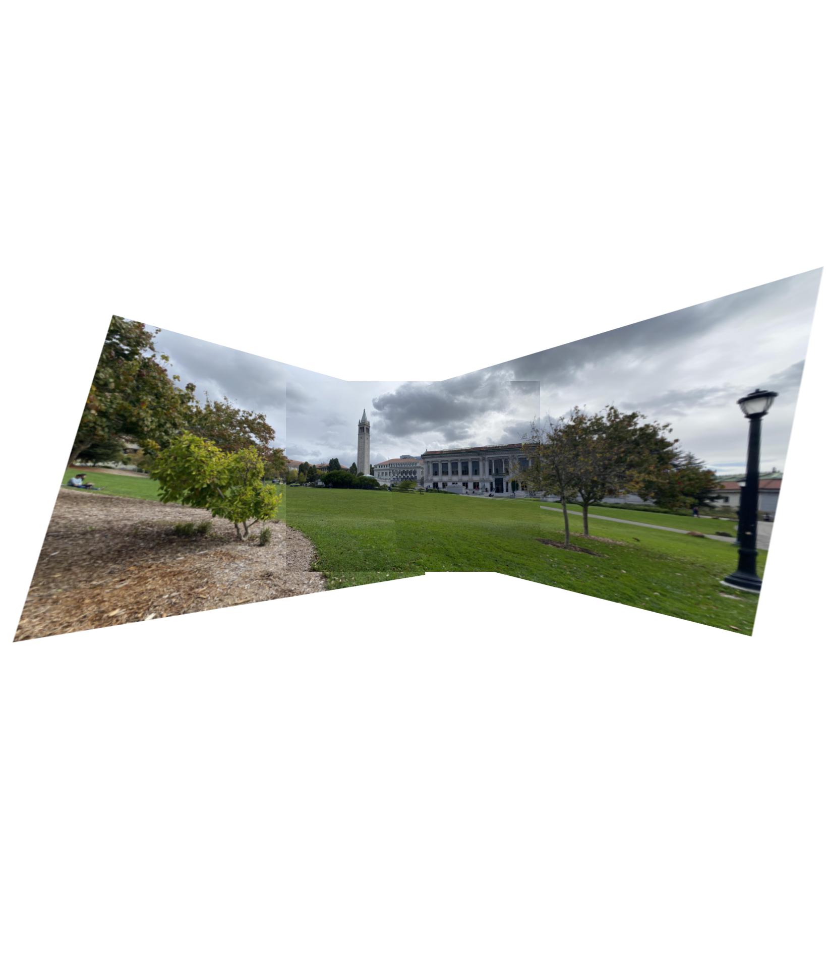 And warped this image into cylindrical coordinates:
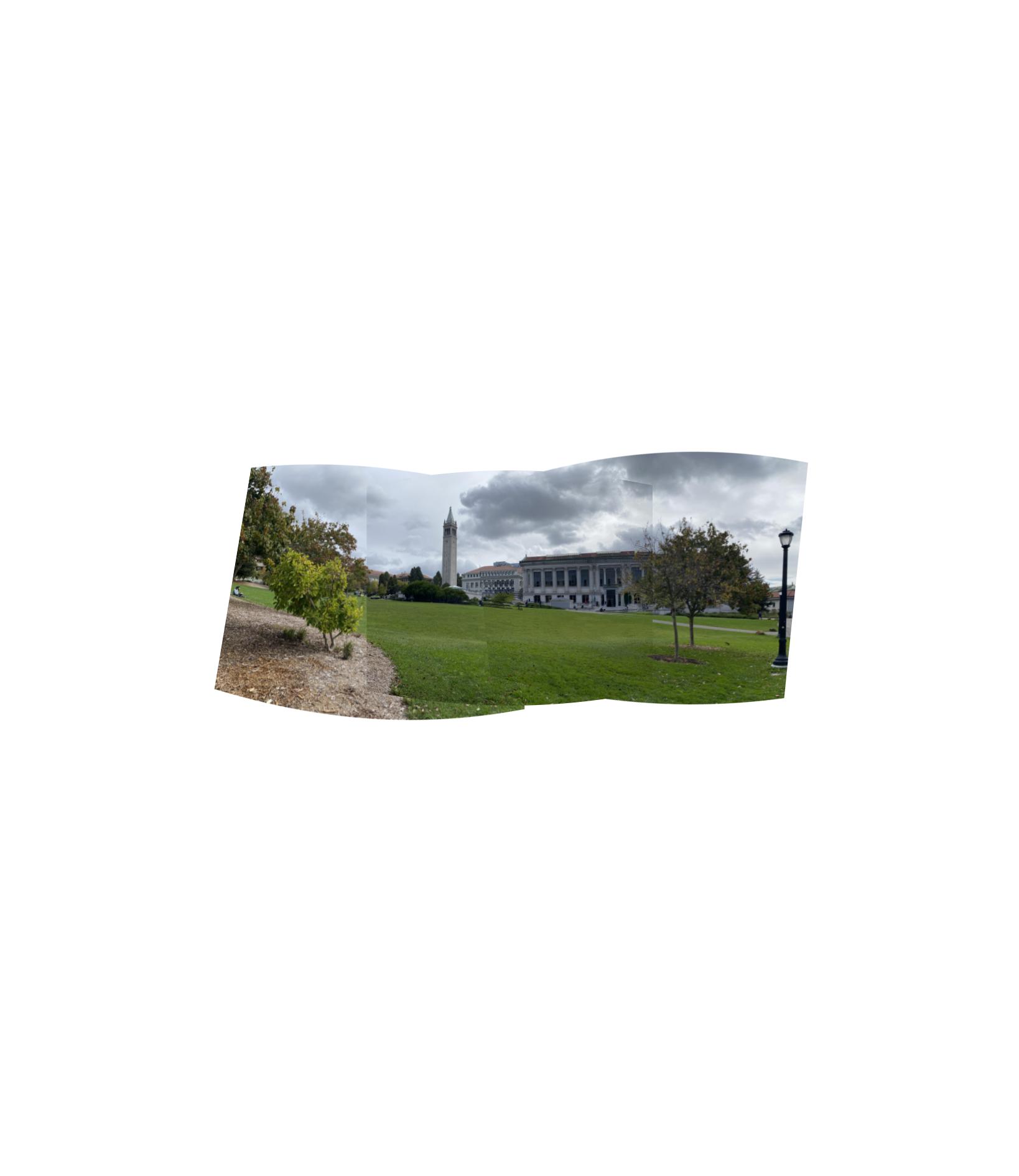 That looks much more natural. The cylindrical warp was interesting to write because it was quite similar to the inverse warp using a homography. Instead of using a homography to transform the image, however, I used the intrinsic camera matrix K with parameters for focal length and the image's center.
Part B Reflections
This was the most challenging project for me so far, but also the most fascinating. It was amazing how well the automatic keypoint detection method performed, outperforming manual labeling in some cases!