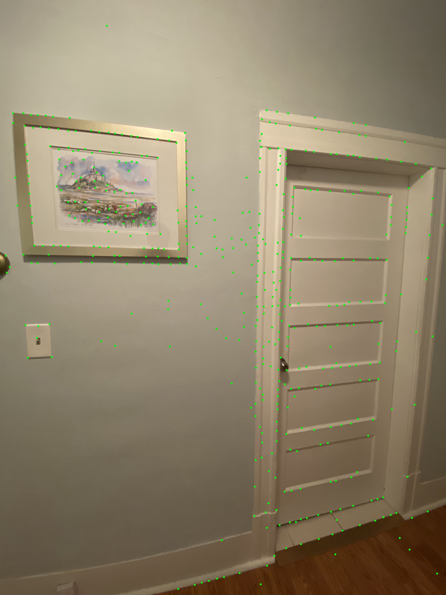
Top 500 points (raw f) 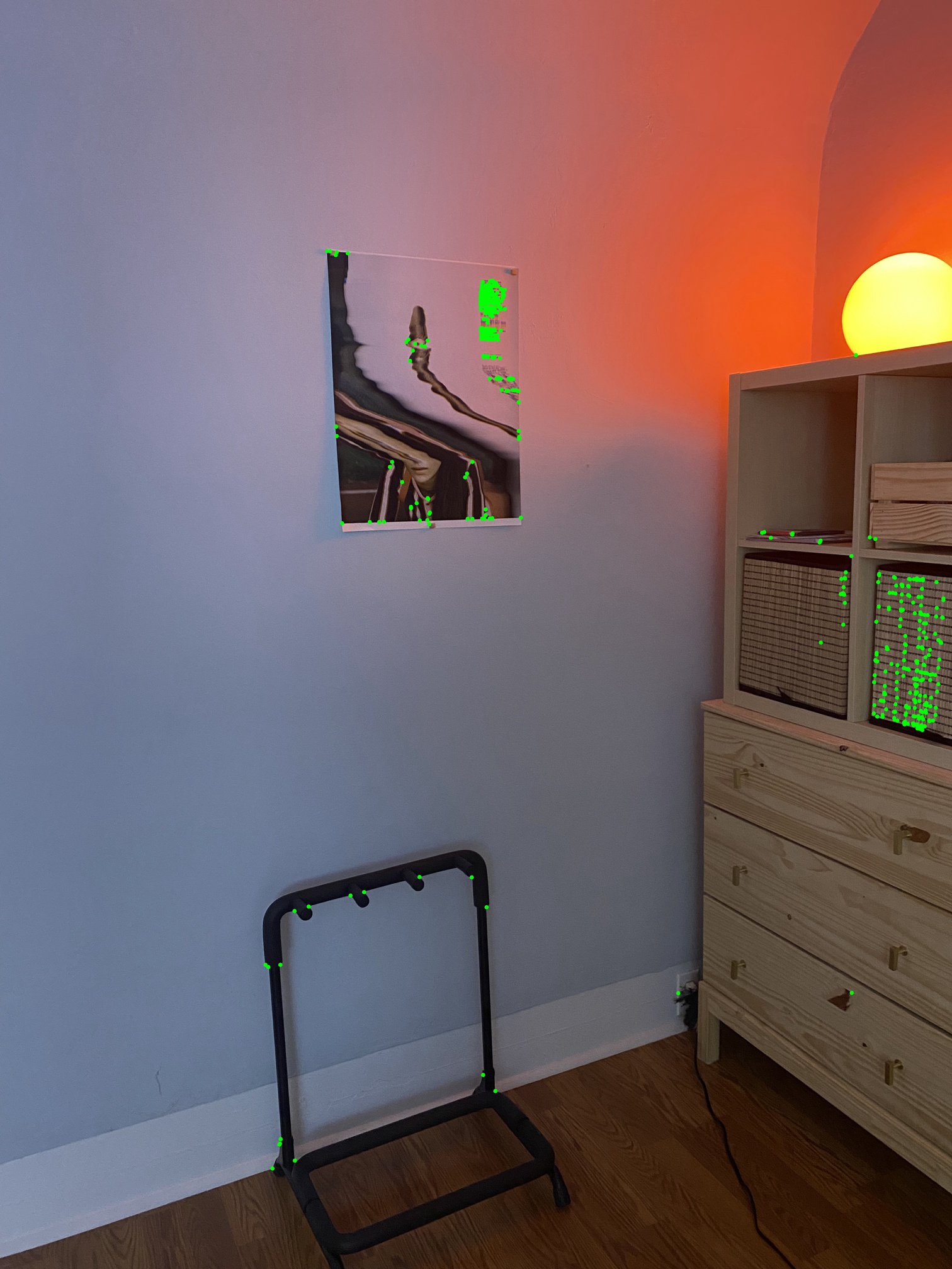
Top 500 points (ANMS) 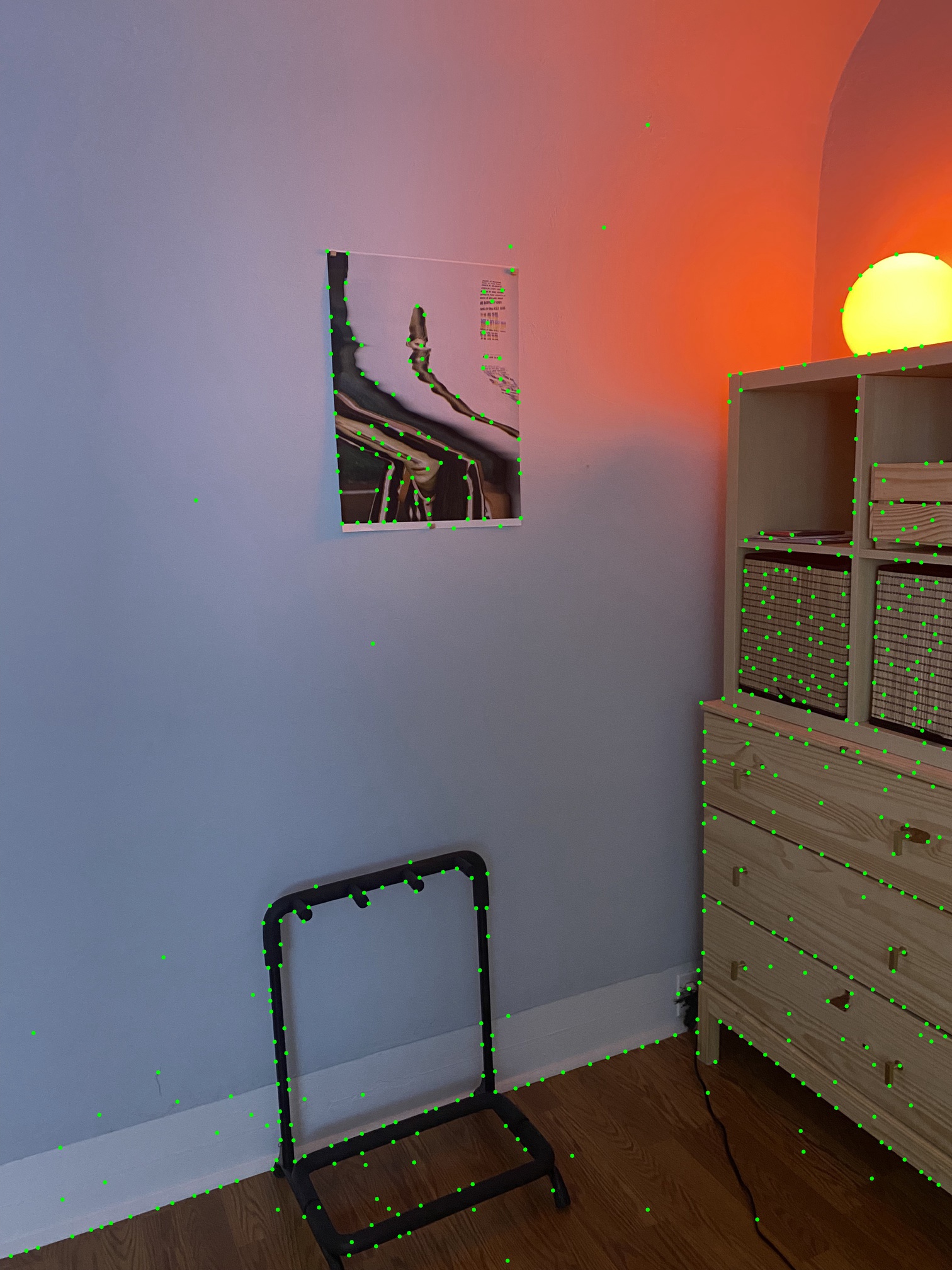
Feature Matching for Auto-stitching
Jeremy Warner — jeremy.warner at berkeley.edu
Using the harris.py provided code, we compute the corner strength map as well as the list of candidate feature points sorted by their strength. To goal is to mix selecting points that have good spatial distribution along with high corner strength. To achieve this goal, we use the Adaptive Non-Maximal Supression (ANMS) technique described in the Multi-image matching using multi-scale oriented patches paper from CVPR ’05.
The minimum supression radius ri is given by: ri = minj|pi−pj|,
where f(pi) < crobust * f(pj), pj ∈ Image, and parameter crobust = 0.9.
Additionally, i and j represent indices of points of interest in the image, and f(pi) is a function that returns the Harris corner feature strength for a given point in the image.
Given the list of points is already sorted by their corner feature strength, we can then find the distance to the nearest stronger (or comparable) neighbor. r[0] is given by Infinity. We then choose the top N points based on this distance to stronger neighbors.
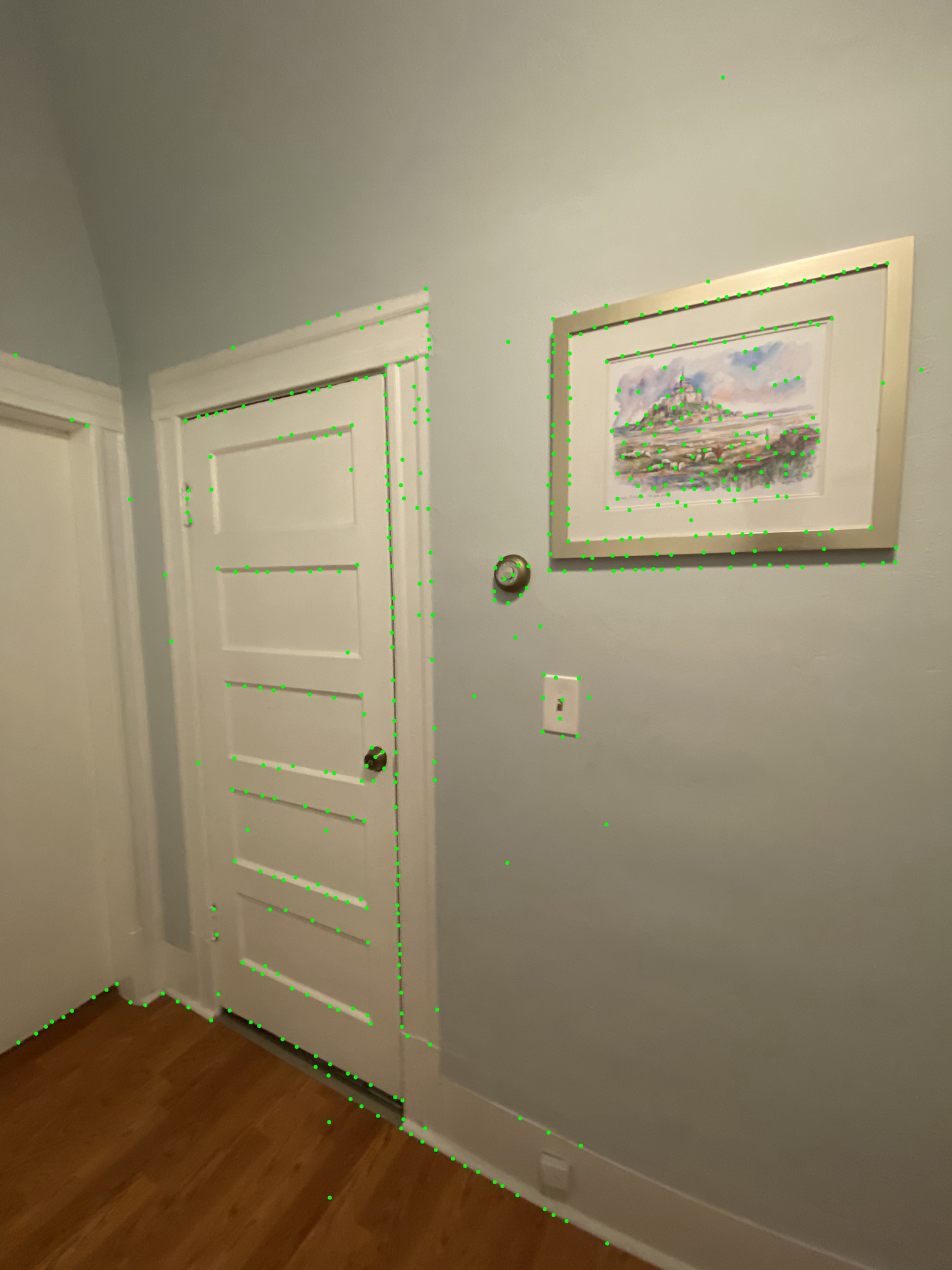
The ANMS method has clearly higher spatial distribution of corner candidate points. Another marked scene:
For each point of interest that we calculated in section 1, we now want to generate a feature descriptor that can be used to correlate points across related images. To do this, we will first take a 40 x 40 grayscale patch centered on the point of interested. Then, we blur and downsample to get an 8 x 8 patch, and apply bias/gain normalization.


Using the sum of square differences (SSD) method for patch comparison, we first compute a similarity score table with a corresponding row and column for each of the normalized feature patches computed in step 2 (500 x 500). We take advantage of Lowe’s rule regarding the error ratio eNN1/eNN2 to compute the ratio between the error of the first (best) match and that of the second-best match.
The smaller this ratio is, the more selective the matching of points will be. We filter the table of patch similarity along both the row and column axes based on the error ratio threshold, performing a union of unique point matches from the perspective of both images we are trying to match across. Finally, we filter out all points that have matched to multiple other points in the other image with a uniqueness check.
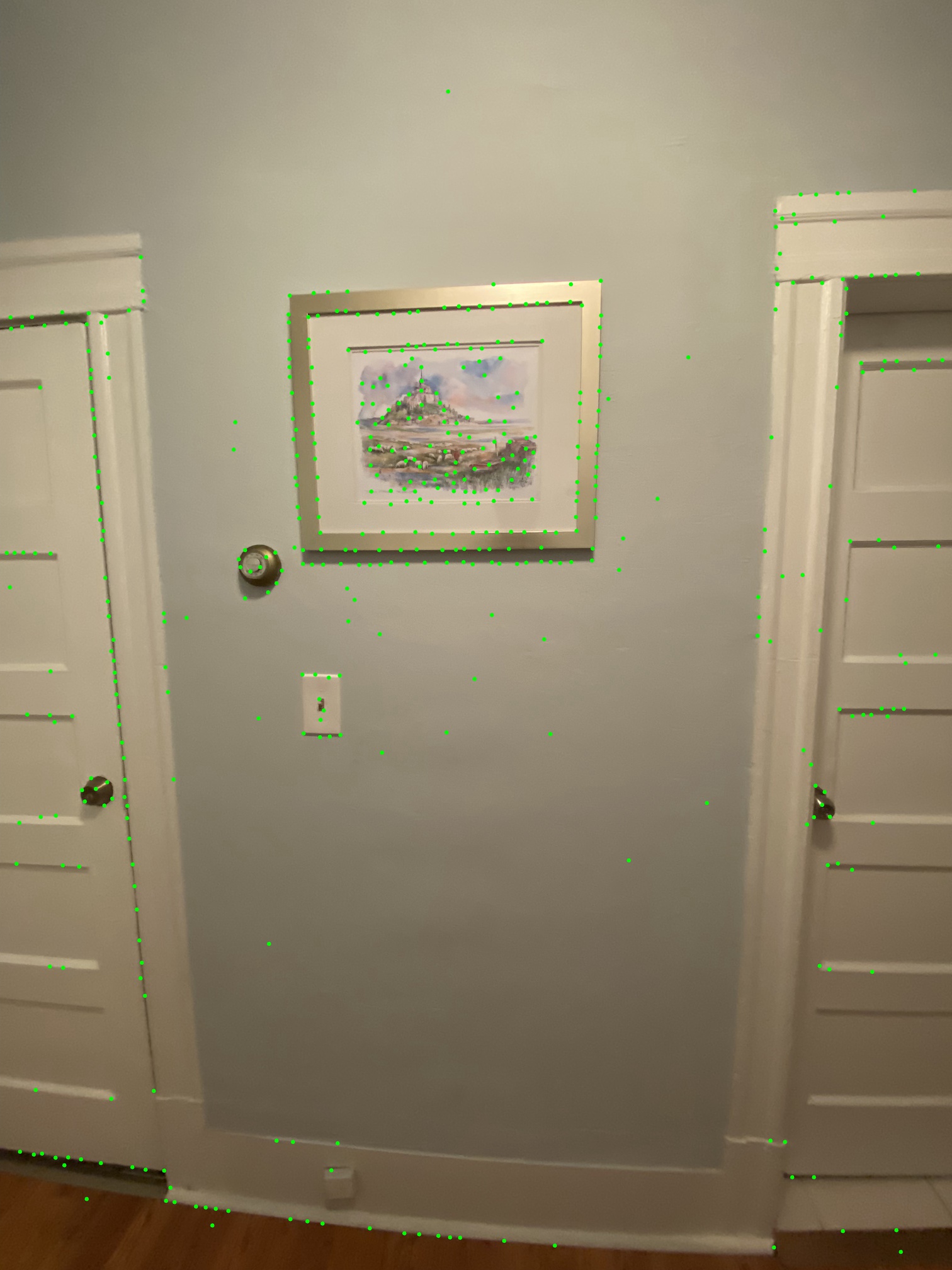
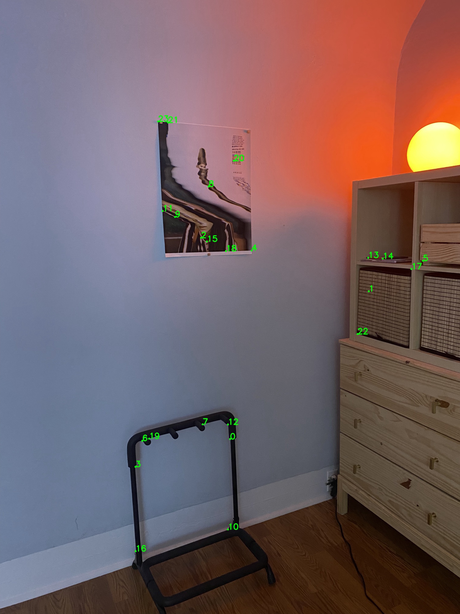
Candidate feature match points (57 pairs from 500 POIs):


Assuming that all of these points were correct matches this far, we could reuse the Least Squares homography estimation technique from Part A. However, it is clear only a subset of points were successfully matched with the patch-based feature matching from this part. The least squares solution is heavily influenced by outliers, so that won’t work well here. Instead, we can use randomized sampling consensus to get the homography instead.
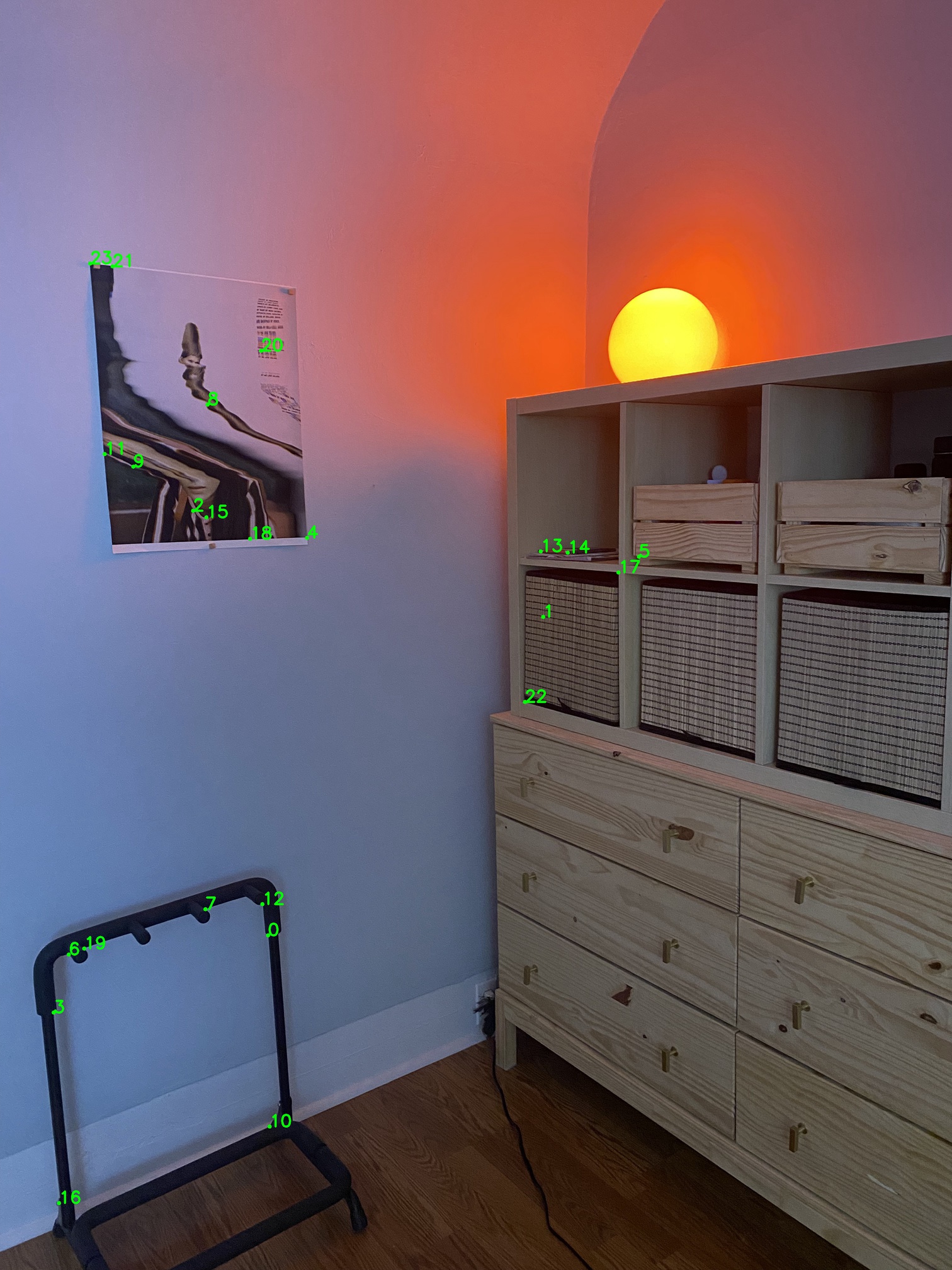
Computing the homography with RANSAC involves taking in the paired points and a fixed number of iterations. The algorithm works by iteratively selecting four random pairs of points and computing an exact homography H. All candidate point pairs are projected with this H and then filtered based on if they fall close (dist < ϵ) to their marked pair. This method allows us to estimate a robust homography from a dataset that has clear outliers.
RANSAC Filtered points (23 final pairs):
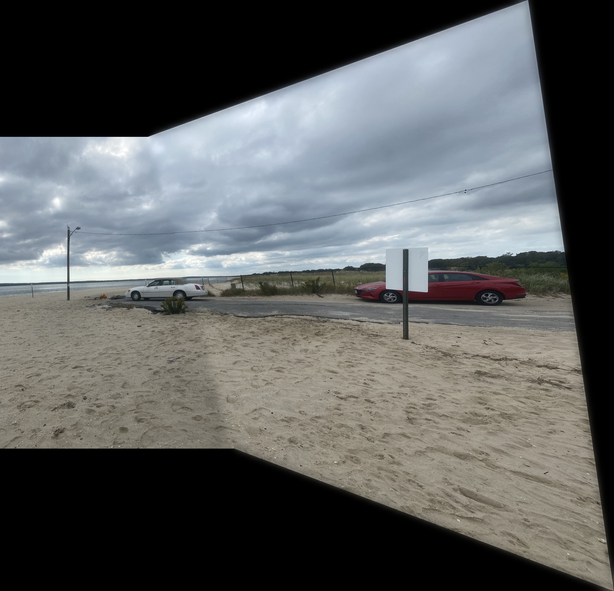
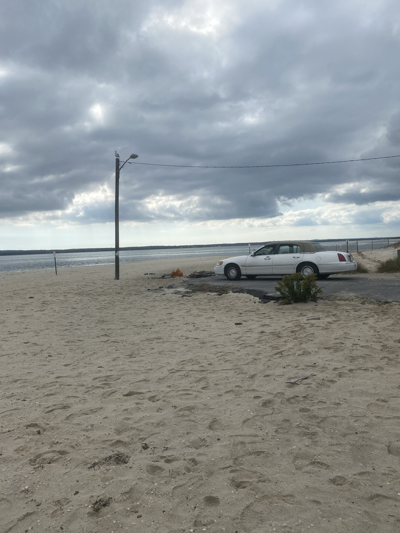
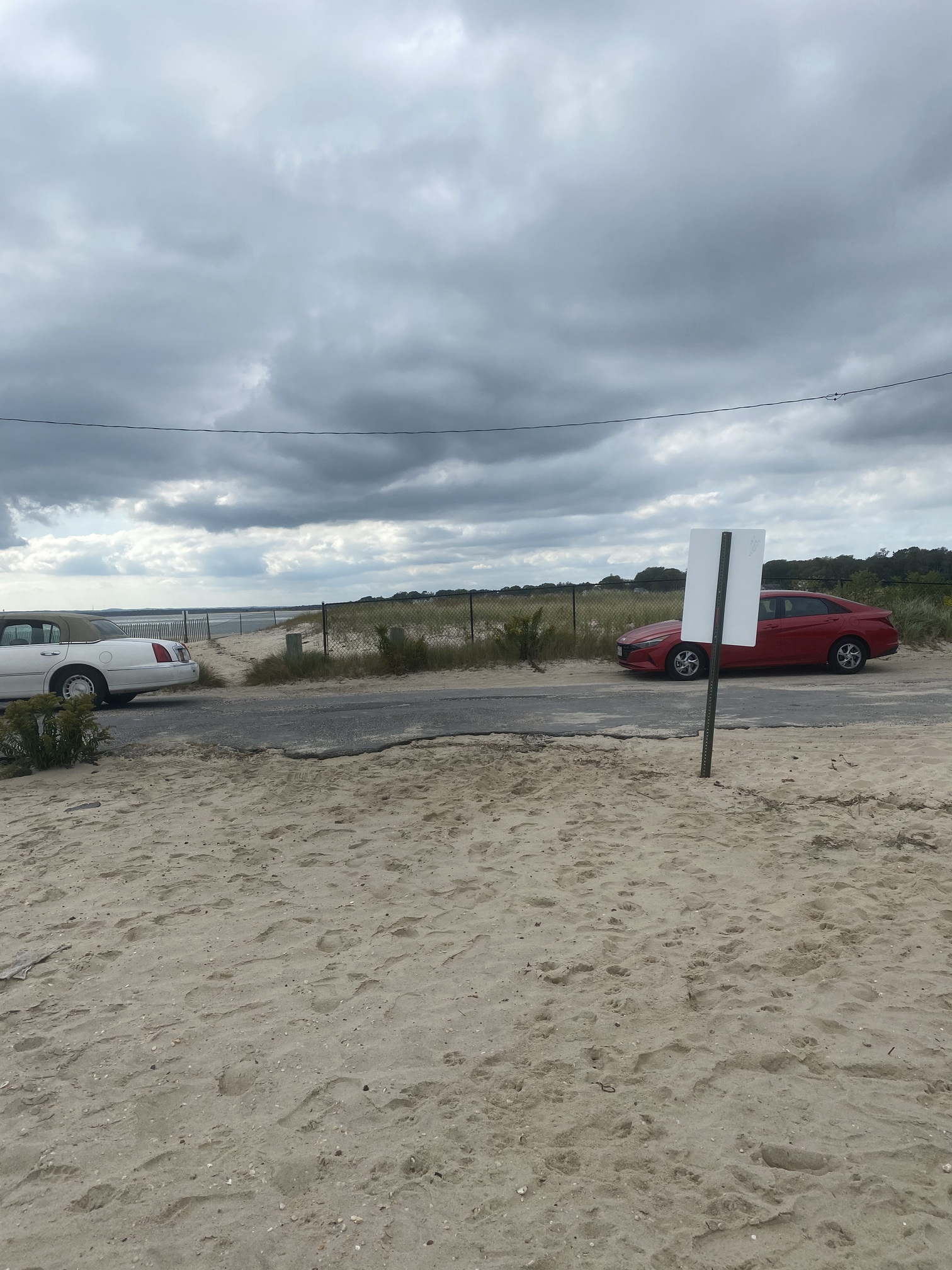
Using our automatic techniques, we compute homographies for scenes using only the input image sequences. Mosaics are then produced using these homographies with the previous image blending functions from Part A. These were all generated using 10000 iterations of RANSAC, running ~1 minute per auto-stitching scene.
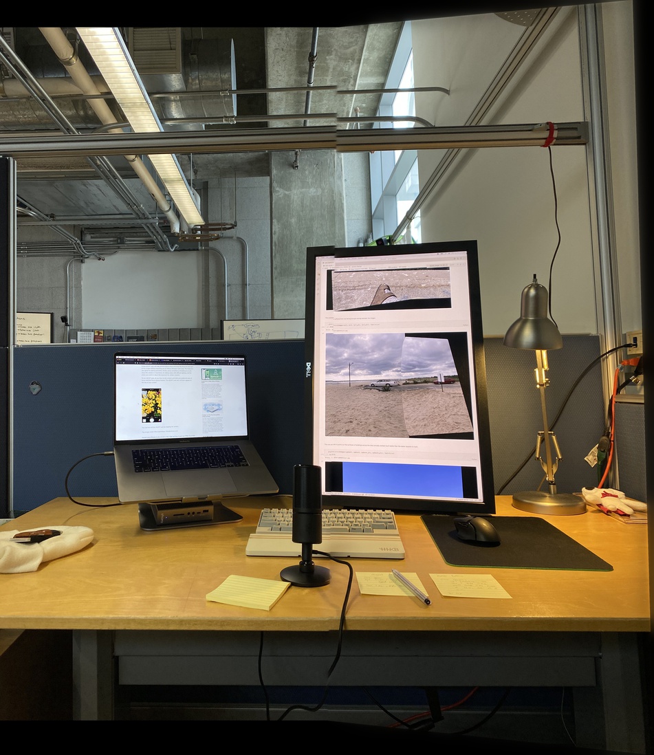
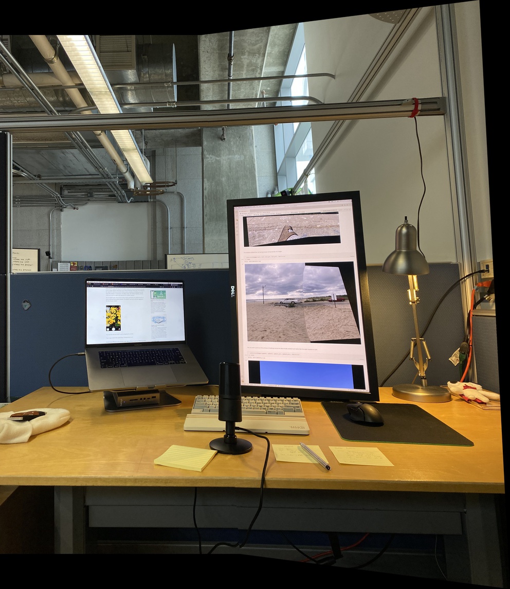
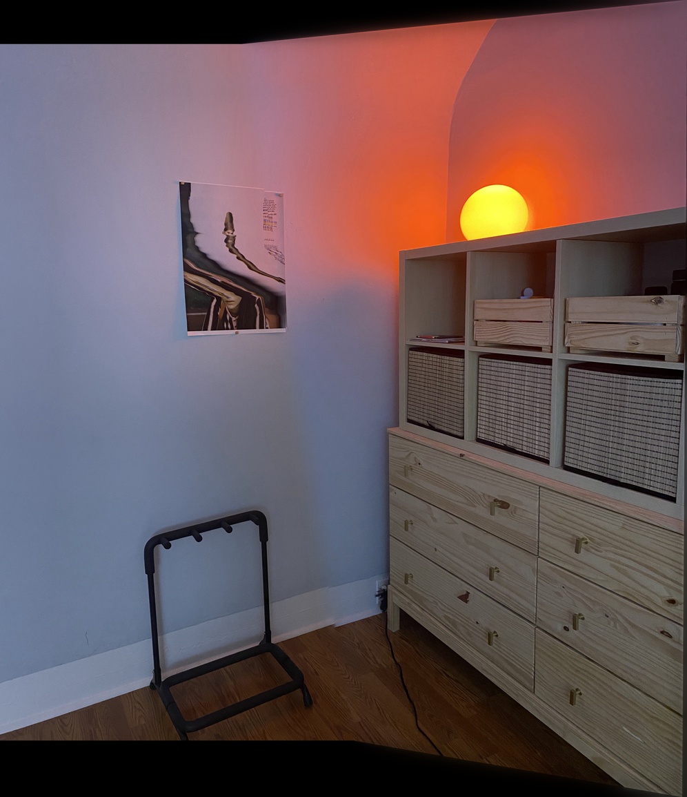
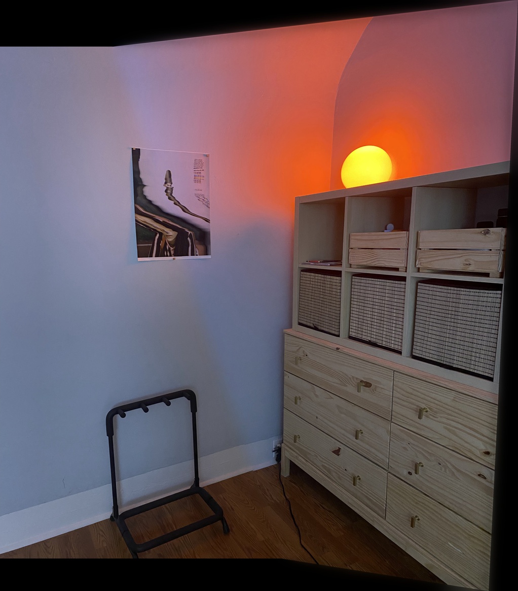
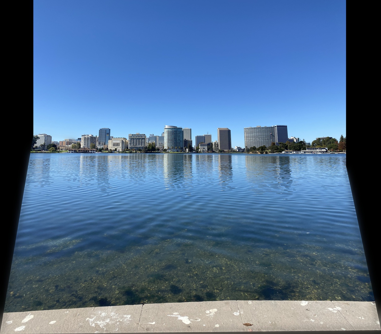
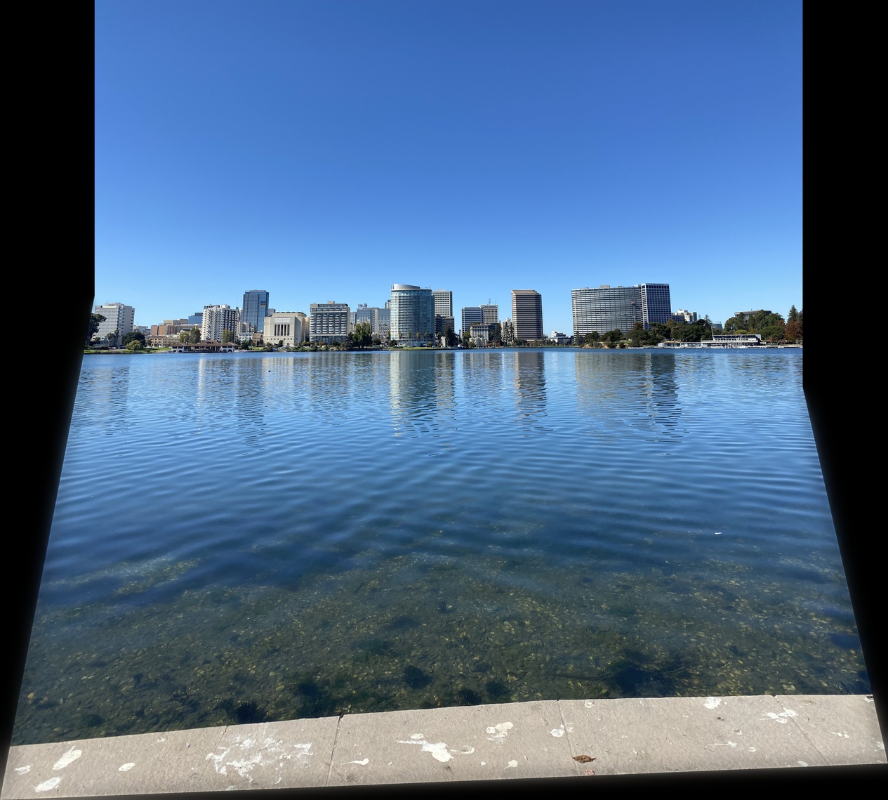
Blending images with a small amount of overlap works surprisingly well, though I did have to increase the number of RANSAC iterations to 50k before I got a nice result. Performance-wise, this stitching took just under three minutes. I tried to select several points to use this as an example for Part A, but it didn’t work. The automatic approached seemed to handle it just fine, with a bit of patience.
This project was challenging, and a ton of fun. It’s amazing to see how composable the different techniques for image alignment were, from using the image blending and warping projects. My favorite part of this project was learning about RANSAC, and seeing how quickly it was able to automatically handle the tedious problem of selecting corresponding points between images.