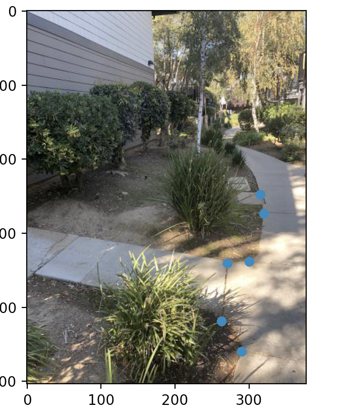
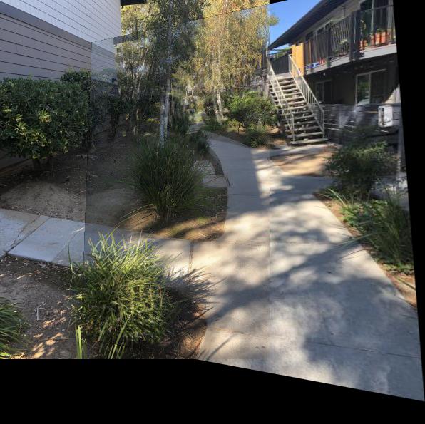
Shoot the pictures
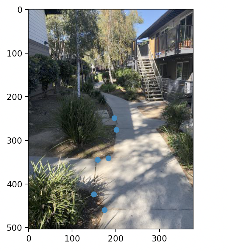
I took pictures with my phone of places outside and some scenes indoors. Then, I labeled the correspondences.
Recover Homographies
To compute the homography between 2 images, I passed in 2 sets of correspondence points. Denote these as pts1 and pts2.
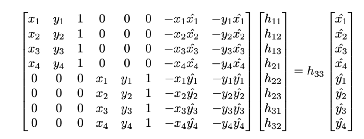
We want to compute the homography matrix that transforms pts1 to pts2. I constructed the following matrix using pts1 and pts2,
where pts1 = (x, y) and pts2 = (xˆ, yˆ). I solved for the h vector, appended a 1 to it since we can just set h33 to 1, and reshaped it into the 3x3 homography matrix H.
Warp the Images & Image Rectification
We warp the images by selecting a target image that we want to warp to. We do this by selecting points shared with 2 images
and computing a homography then warping one image to the other with the homography by applying it to that image's coordinates.
Then, for each pixel in our final image, we find where it comes from in the source image using the coordinates and interpolate to get the value.
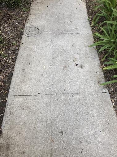
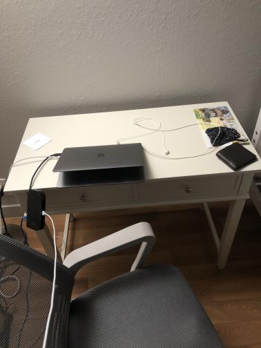
For rectifying, we can just select 4 points to be a bounding box on a plane in the picture, such as the 4 corners of a table,
and we can warp to that plane to get the top-down view shown below.
 Initial
|
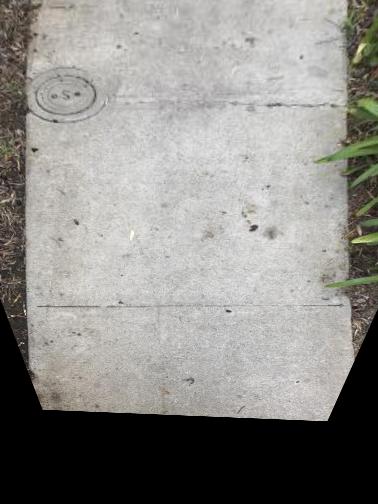 Rectified
|
 Initial
|
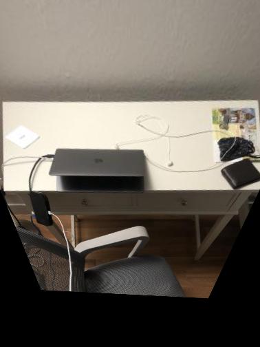 Rectified
|
Blend the images into a mosaic
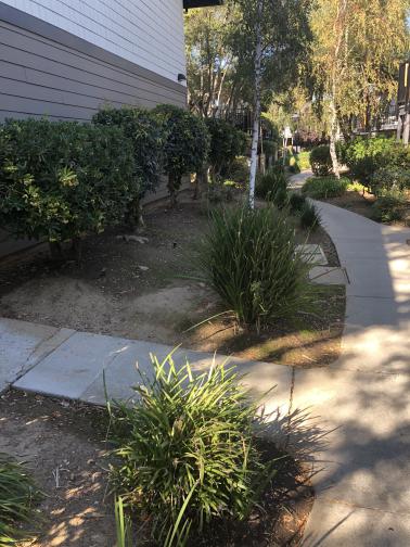
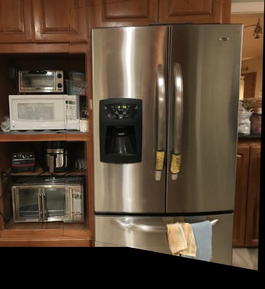
Now, we can blend images. I selected a couple of images, where I warp one of them to the other using the homography, and stitched them
together into a mosaic by doing a weighted average of the overlapping region of the images, which I found by
creating boolean masks of the images and seeing where the product is 1.
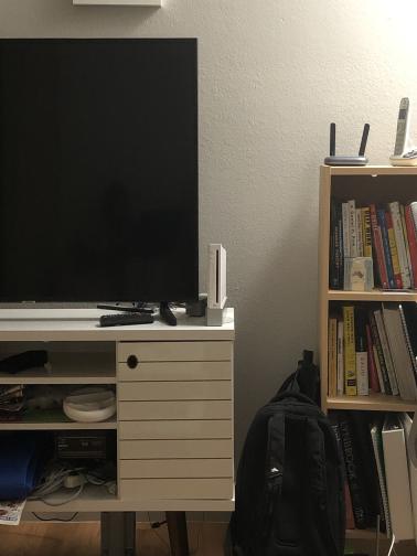
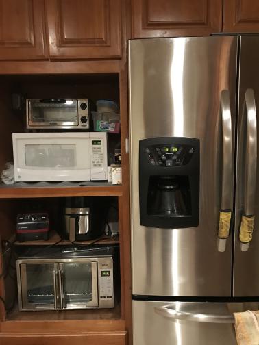
 First Image
|
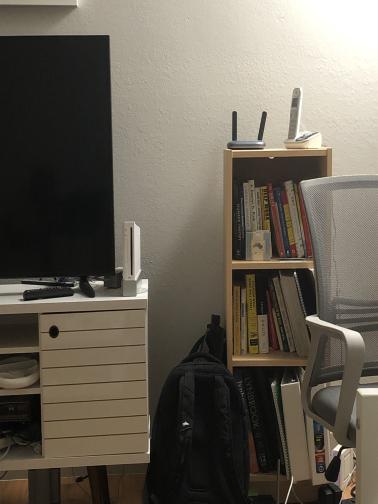
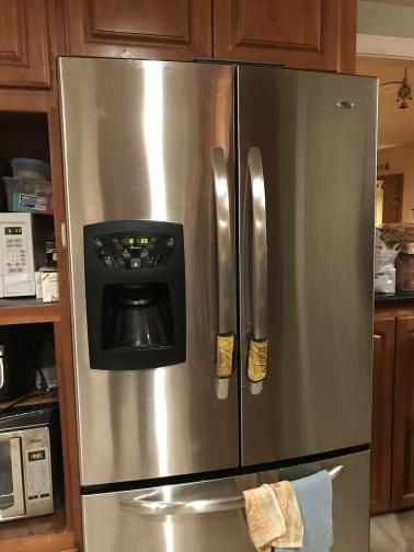
 Second Image
|
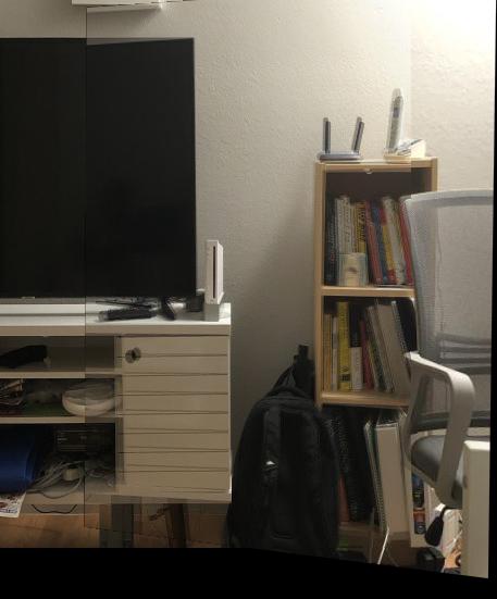
 Mosaic
|
 First Image
|
 Second Image
|
 Mosaic
|
 First Image
|
 Second Image
|
 Mosaic
|