Scroll down for Project 4B.
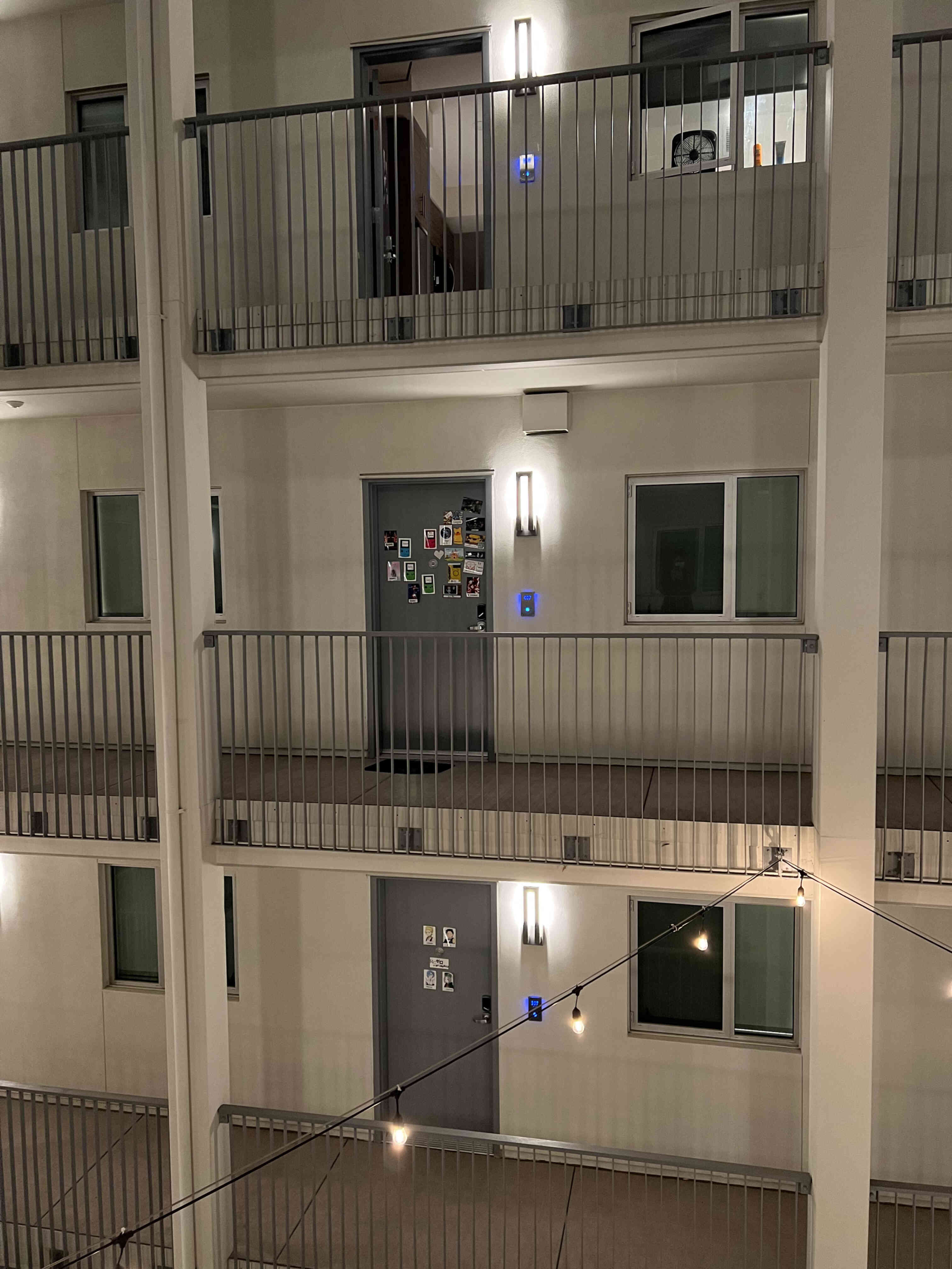
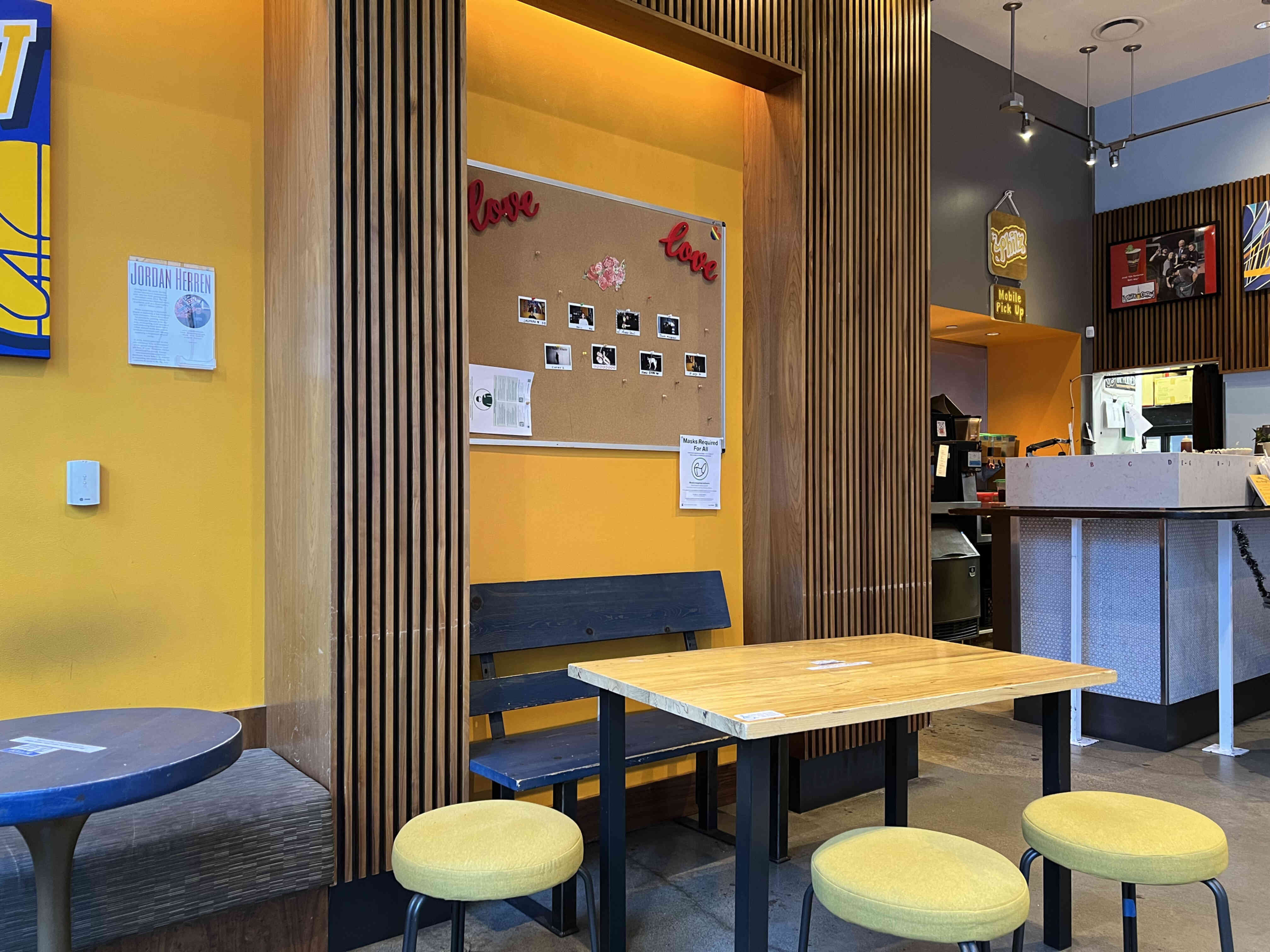
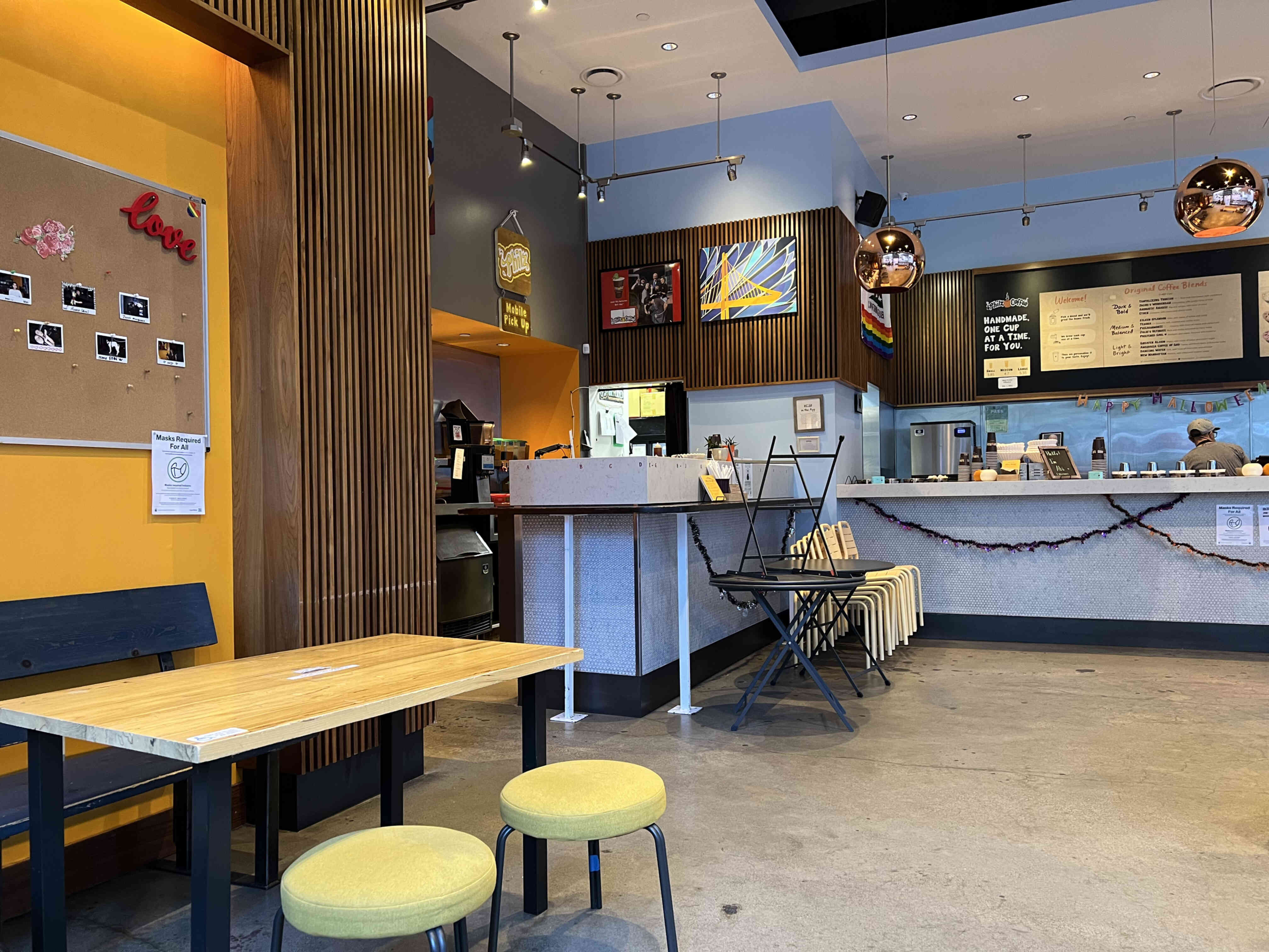
Shooting Scenes
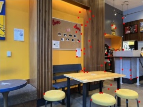
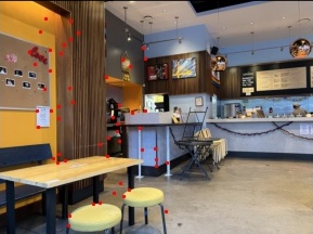
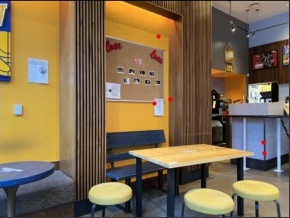
Recover Homographies
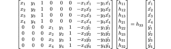
The goal of computing a homography is to solve the equation p' = Hp, where p is a set of points on one image and the homography matrix (H) transforms those points into warped points p' of another image. Since this matrix is a 3x3, there are 9 unknowns. However, rearranging this into a system of equations yields that one of the parameters of H is actually a free parameter which can be set to 1 for convenience. The following system of equations was used with 6-8 correspondences per pair of images in experimental results.
Warp the Images and Image Rectification
Inverse warping with the H matrix was used to generate the new scene geometry, and below are some examples of warping being used to rectify an image such that a planar surface is frontal-parallel.
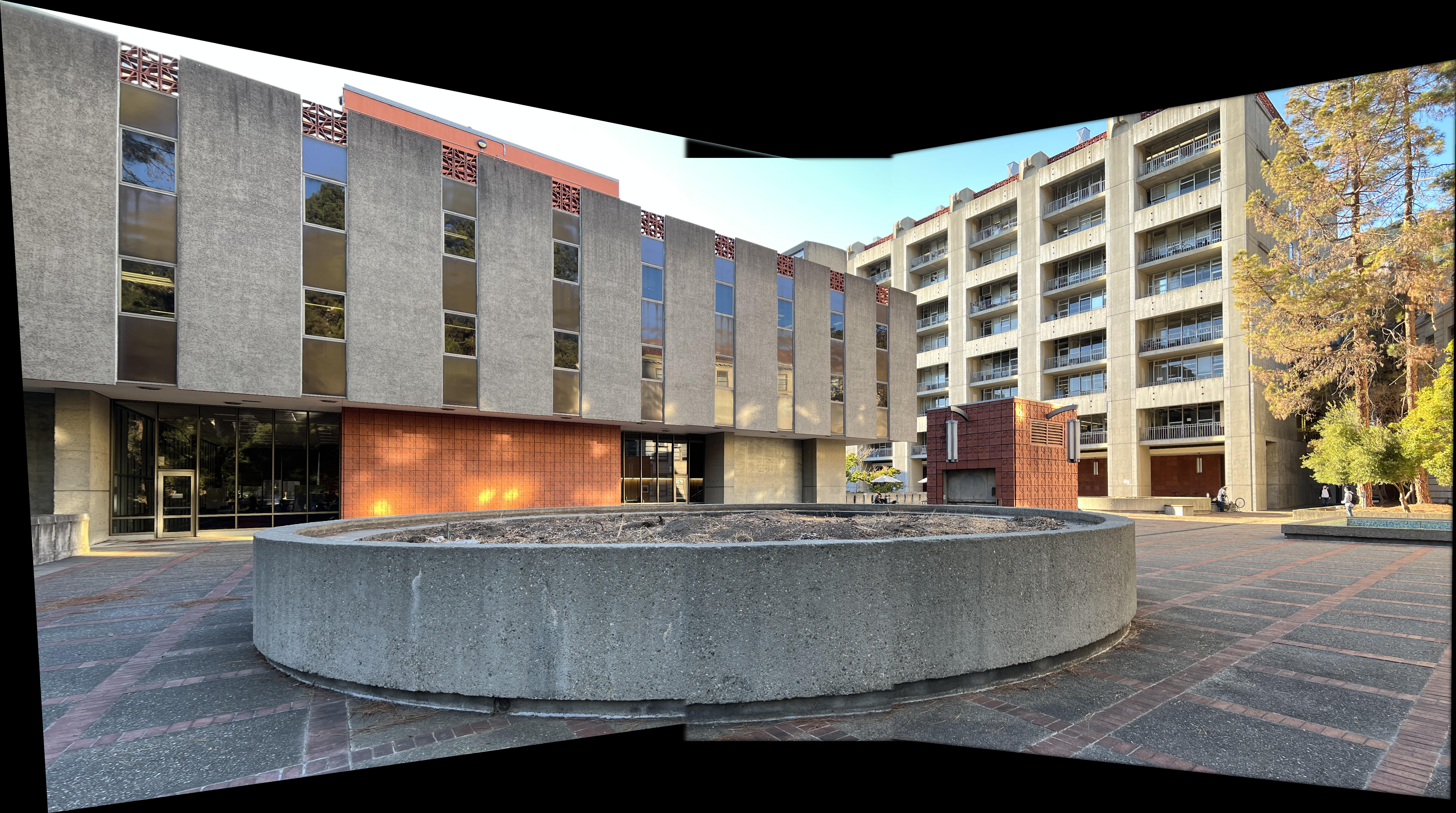
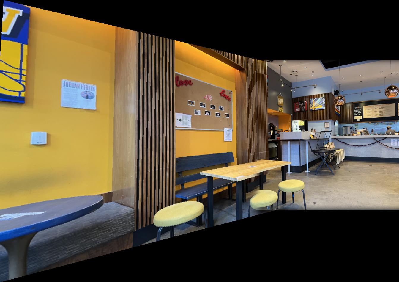
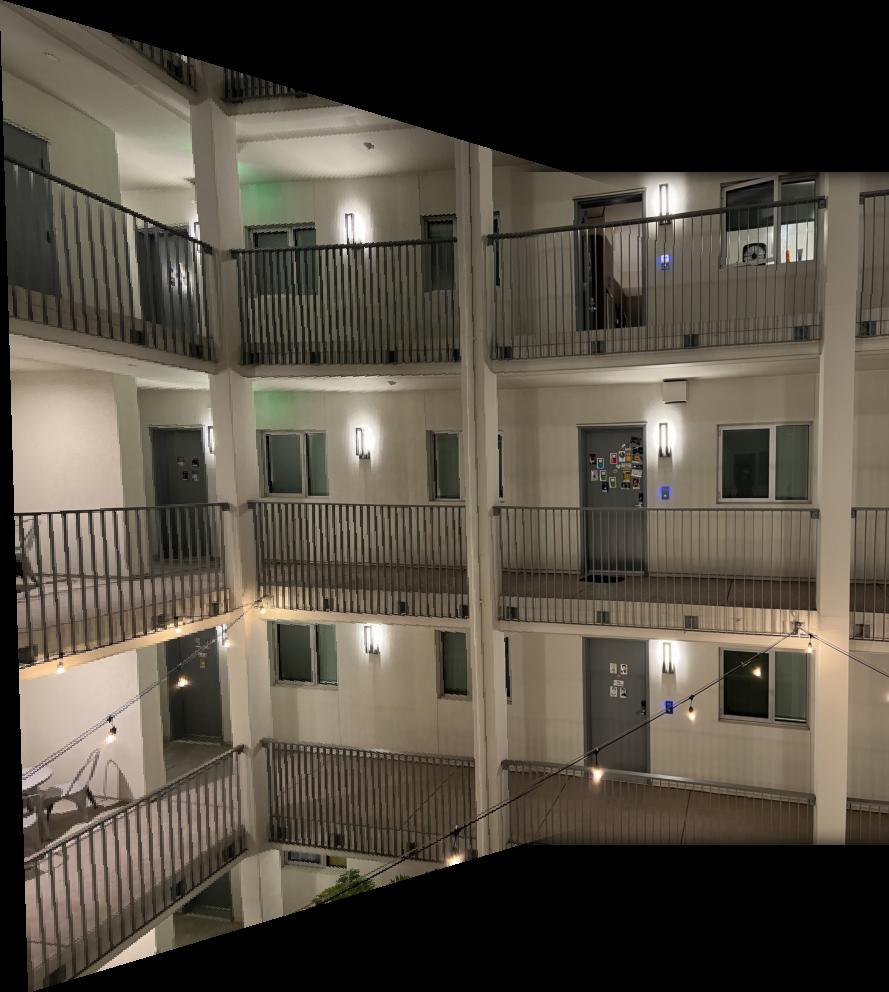
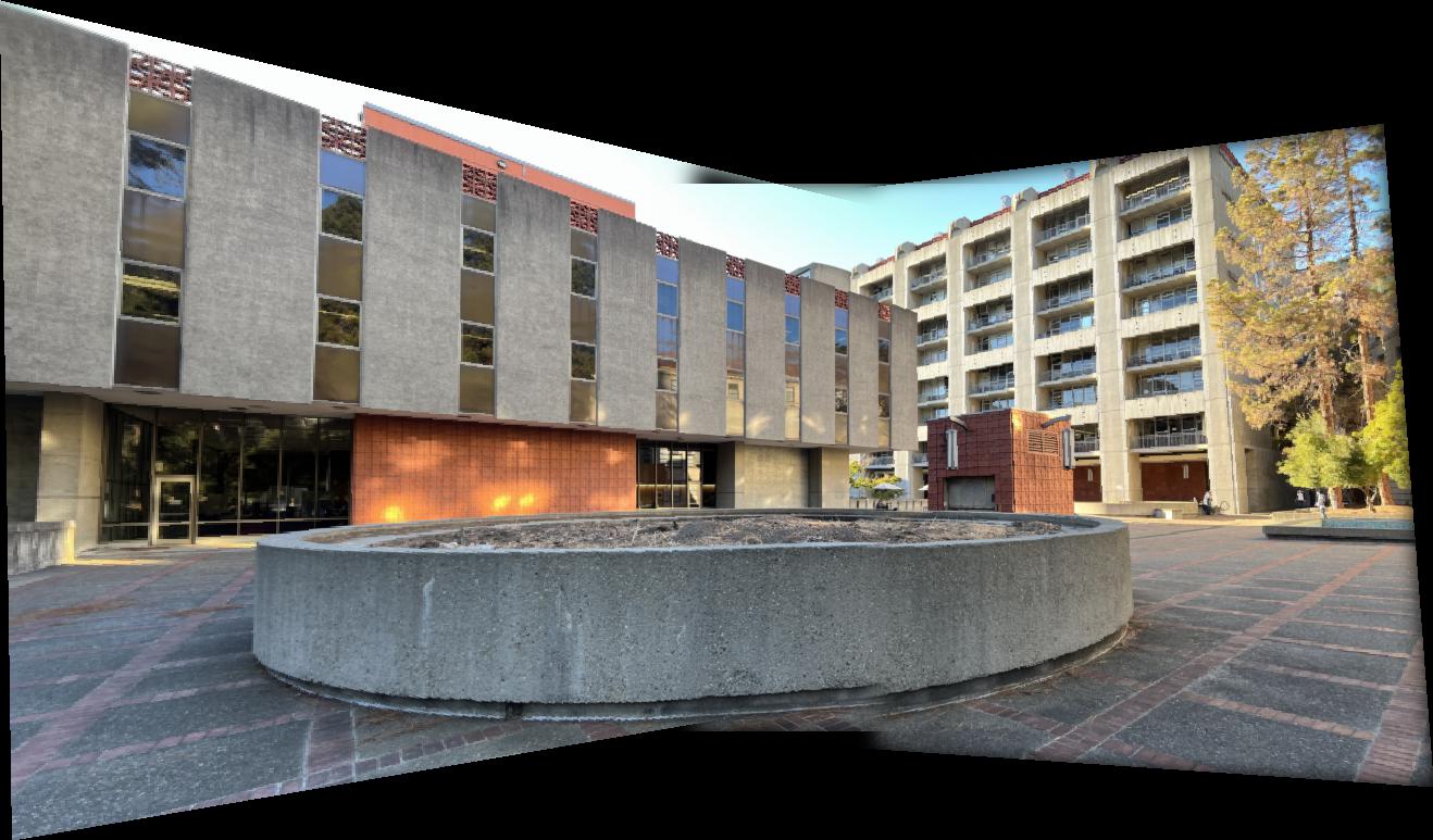
Blend Images Into a Mosaic
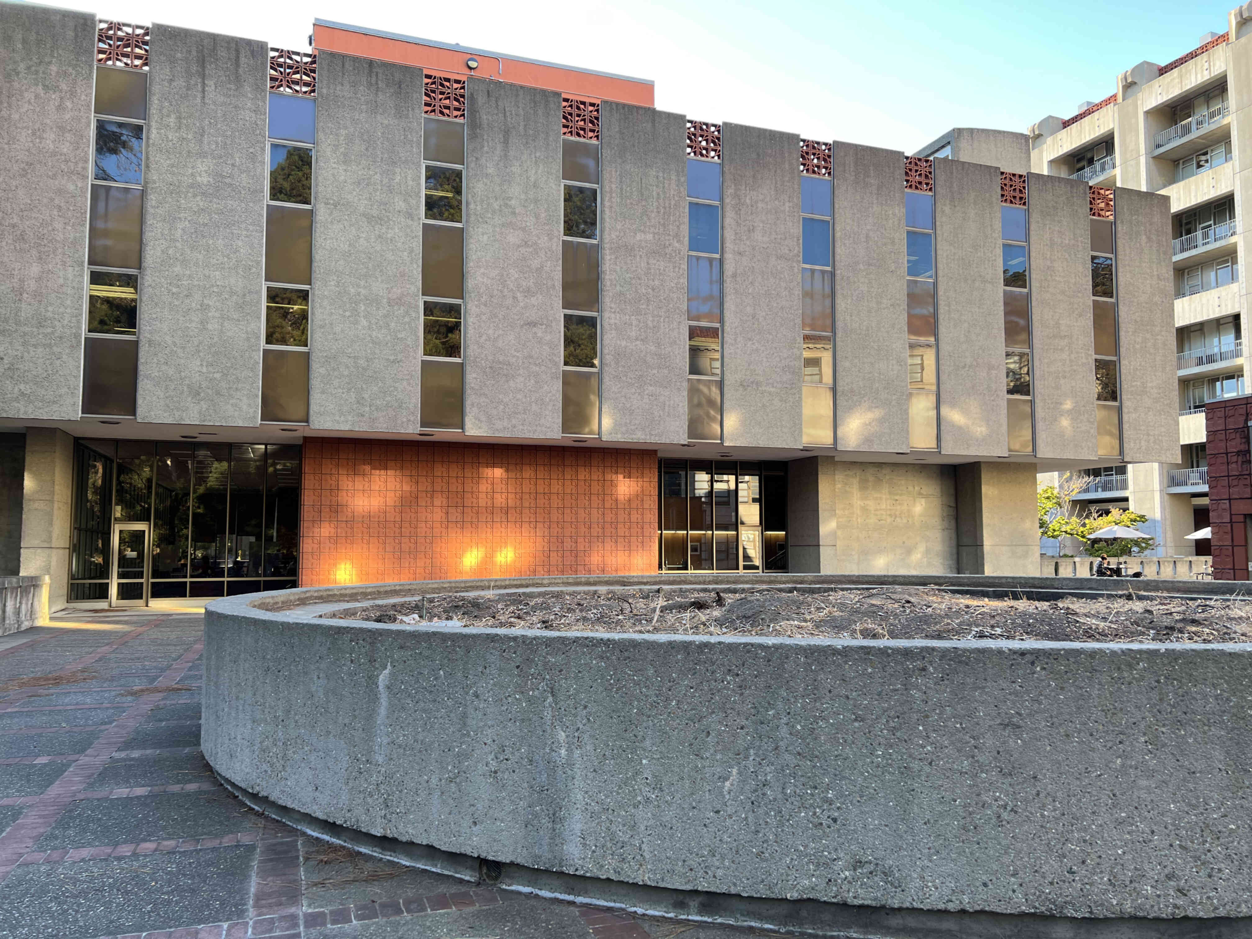
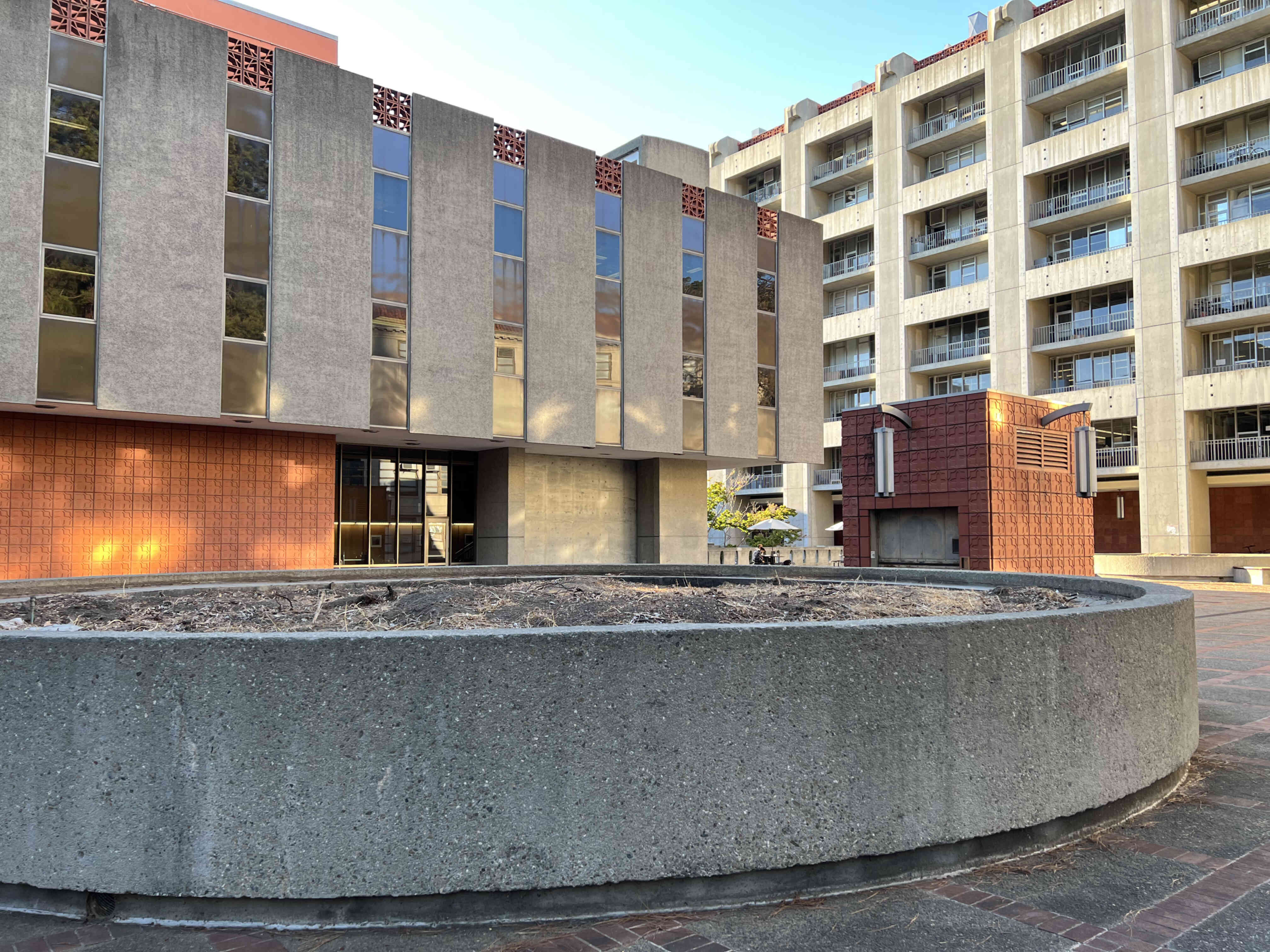
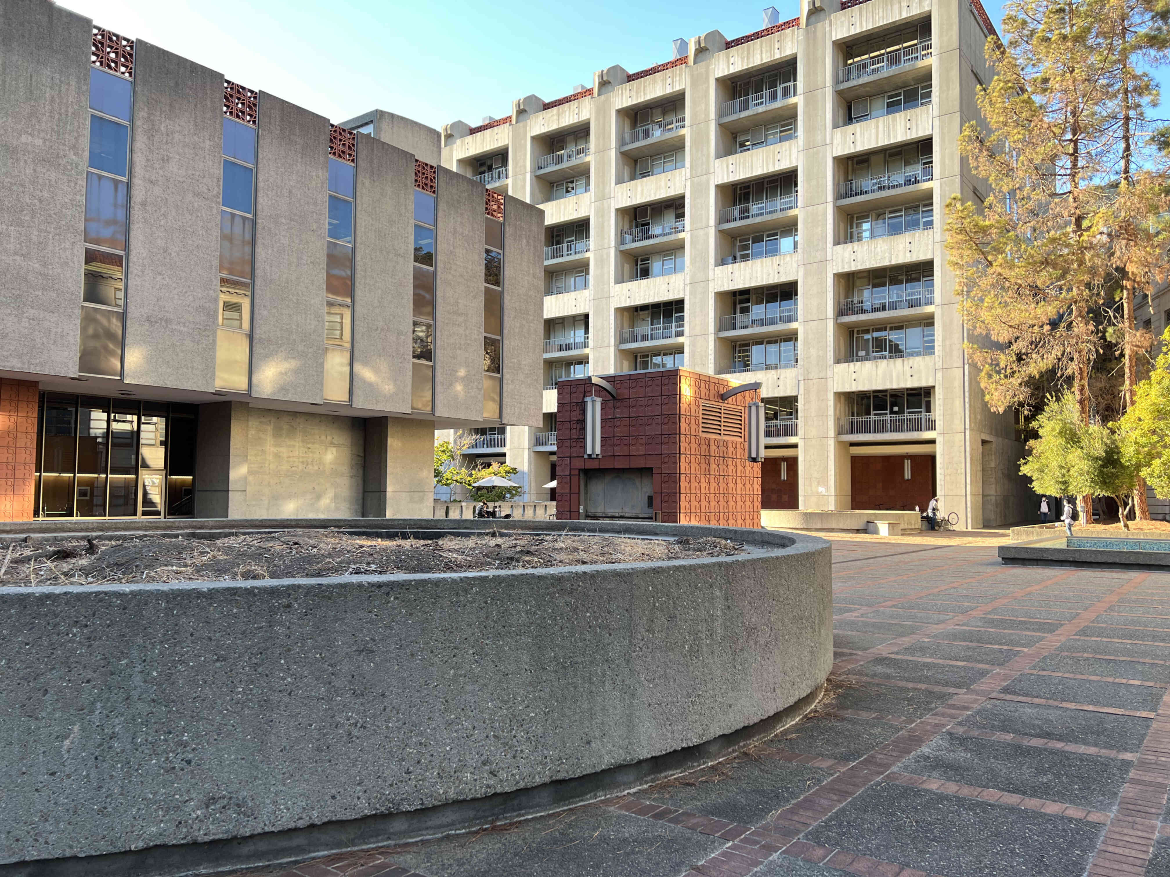
Given a sequence of images, I first set the canvas coordinate system to be a translated version of the center image in the sequence. I then warped each image in the sequence and placed it on the canvas. To smoothly blend between images, I computed the intersecting area between a warped image and the rest of the canvas and used the middle line splitting the intersecting area as the axis to blend between the two images. The blend axis allowed for a smooth transition between images since this axis was blurred with a Gaussian filter. Below are results on three different scenes.
Lessons Learned
I learned how to effectively leverage homography to automatically stitch images with manually assigned visual correspondences and that the algorithm for doing this is surprisingly simple! I also learned a lot about the algorithm's sensitivity to change of camera settings or alignment of correspondences across images (it is not very robust to noisy correspondences or images at this point).
Project 4B: Autostitching
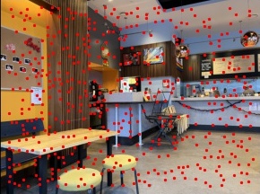
Harris Interest Point Detection
Using the starter code provided, we collect a large number of candidate points of interest.
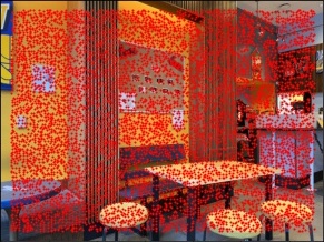
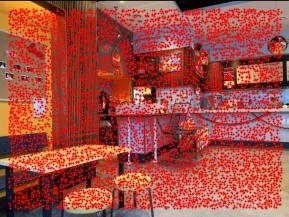
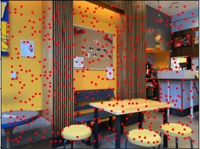
Adaptive Non-Maximum Supression
Using the ANMS technique presented in the MOPS paper, I compute the minimum supression radius for each interest point with c_robust=0.9. The points are then sorted by their minimum supression radius and the top 500 points are kept.
The minimum supression radius for an interest point is defined as:

Feature Extraction and Matching
Feature descriptors are generated by taking a 40x40 window around each point of interest returned by ANMS, blurring the window with a Gaussian filter, and then downsampling to 8x8. Each feature descriptor is standardized to have 0 mean and 1 variance. To match descriptors across images, we compute the SSD between each descriptor and all descriptors in the other image. We use Lowe's trick and only keep a match if the ratio between the 1-NN error and 2-NN error is less than 0.3.
RANSAC
To remove outliers, RANSAC (as described in lecture) is run for 1000 iterations with epsilon=0.1 to find a robust set of inliers for computing the homography.

Autostitching Mosaics
Combining all steps in this process, autostitched mosaics for each scene can be easily generated. Mosaics created with manually-defined correspondences are presented as well for comparison. In all scenes, the autostitched mosaics are of comparable (or better) quality than then hand-created mosaics. The stitching/blending process is identical for both methods (main difference is homography computation).
Lessons Learned
This automatic method is surprisingly effective! The fact that it can produce better or comparable results purely from images is mind-blowing and the simplicity of the implementation is especially impressive. The coolest subpart in this project was RANSAC, which is very simple but very useful for computing a robust estimate from noisy data.