Project 4A

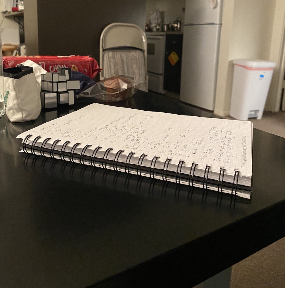
Summary, What I Learned: In this project, I used image warping to create mosaics of scenes from multiple images. I also used image warping to rectify some images to appear frontal-parallel. This was a very interesting project as I got to implement panaorama photos essentially and I learned how to find the homographic transformation between points using least-squares. It was also cool to see how image warping can have applications to information retrieval as I was able to rectify my notebook at an angle, and be able to read the notes after rectifying. Overall, I learned a lot about homographic transformations and how to interpolate warped images.

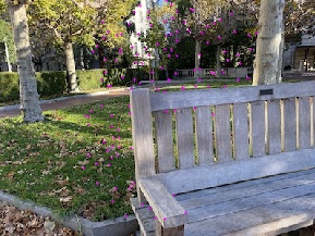
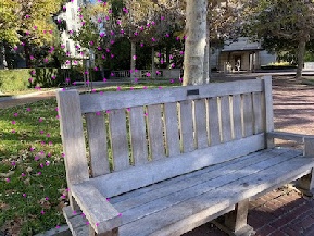
Part 1: Shoot and Digitize Pictures

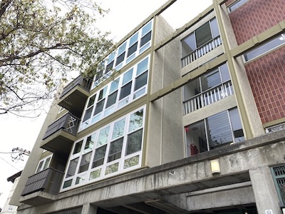
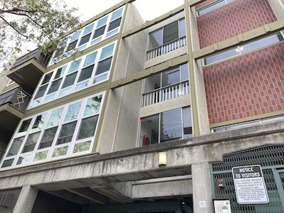
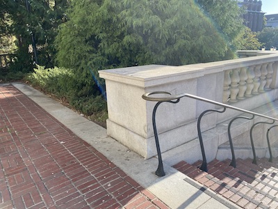
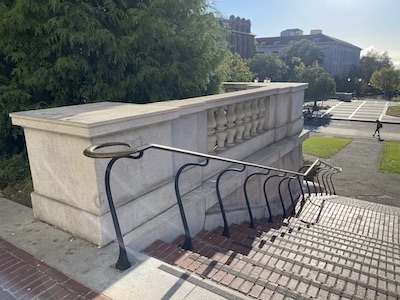
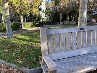
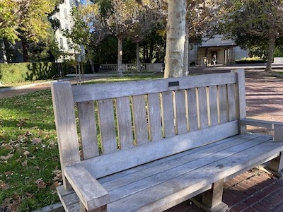
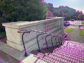
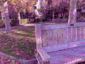
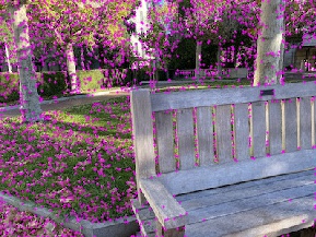
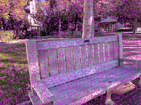
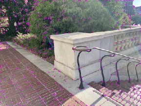
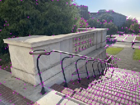
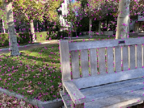
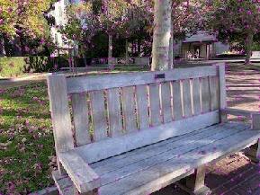
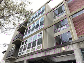
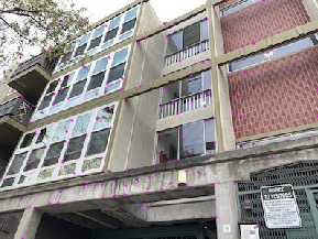
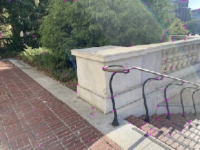
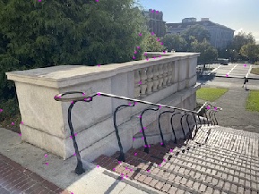
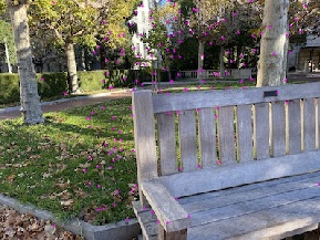
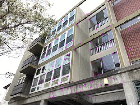
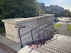
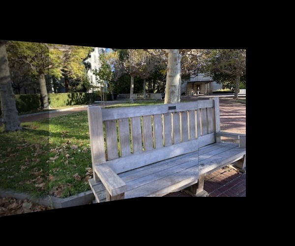
I captured series of images with identifiable geometric shapes. I also made sure to overlap about half of the image between consecutive shots. Below are the three sets of images that I plan to turn into a mosaic.

Part 2: Recover Homographies

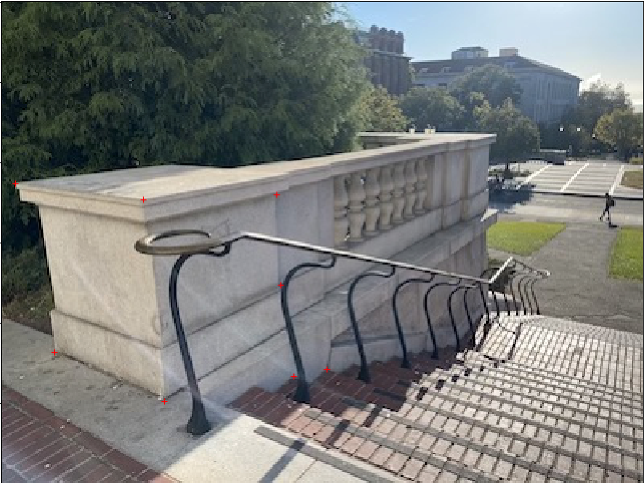
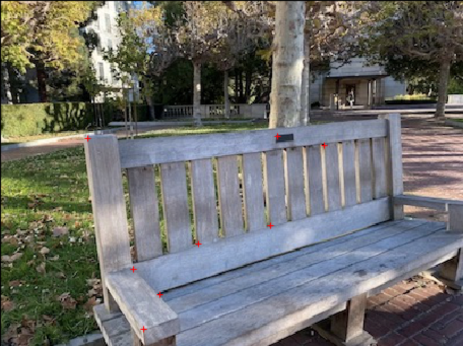
To create the mosaic, I first needed to define correspondence points between the images based on key features. I used 8 correspondence points for each image as labeled in the images.

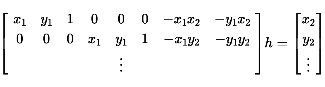
After finding these points, I then determined the homography matrix that maps one set of points to the other. Since this was an overdetermined system, I solved for H using least-squares that would give the solution that minimizes the error. I wrote out the original equations for the homography and then substituted w in. The final result was the following matrix AH = b where b has all the x, y points of the destination correspondences in x0, y0, x1, y1... order.

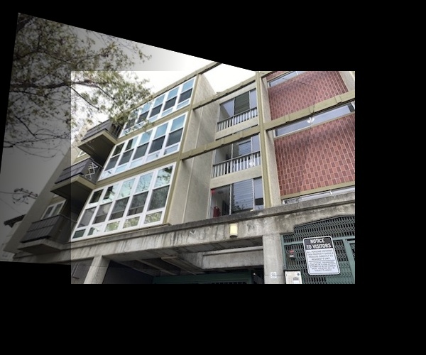
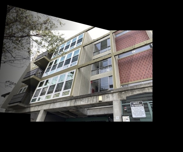
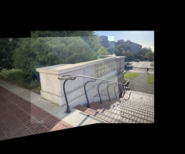
Part 3: Warp the Images

Now that I had a homography matrix defining the homographic transformation between the images, I used the inverse of H to interpolate and map the original pixel values to the new pixel locations using cv2.remap. This transforms the start image so that its shape aligns with the points defined in the end image and the pixel values are interpolated to avoid aliasing. For each set of images, I warped one image to the other image. I made sure to leave room for the second image to be blended in the next step.

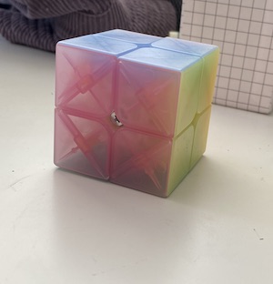
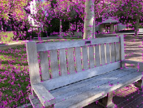
Part 4: Rectify Images

The process of rectifying an image warps a rectangular surface so that it looks frontal-parallel even if it is a different perspective in the image. I did the same process as warping an image by first computing the homography from least squares. I defined four correspondence points at the four corners of the blue face on the Rubix Cube and the four points on the notebook. For the other set of points to warp the image too, I created points of a square/rectangle based on how the ratios I estimated of the sizes and how large they would be frontal-parallel. For example, the cube I used square points of [[50, 50], [200, 50], [200,200], [50,200]]. My final results turned out very good as I was able to rectify the images. It was interesting to note that this also magnified any nonuniformity. For example, the cube edge originally was not totally straight since the face has two multiple surfaces, so you can really see that when rectified.

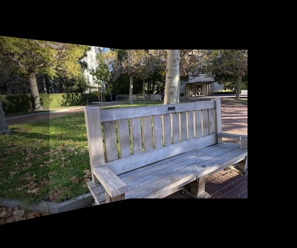
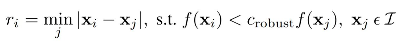
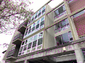
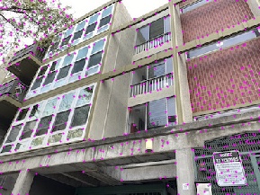
Part 5: Blend Images into a Mosaic

Now that I had my warped images, I blended the two images together in each set to create a mosaic. I translated the both images to leave room for the other image to be added in for my final canvas size. I found the just a weighted average was too abrupt. Instead, I added an alpha channel that would be transformed with the original image where the edges are more transparent. The final pixel values would be weighted by the alpha channel so the edges are more blended.

Project 4B

Summary, What I Learned: For the second half of the project, I continued off of the methods in 4A, but this time did not do the painful task of selecting good correspondence points between images and instead automatically detected corners and found the best correspondence points to warp the image. I thought it was really cool how accurate the results would be and are just as good if not better than when I selected the points myself. After making the initial algorithm procedure, it was much faster to automatically select corners so I find it really amazing how this procedure can now be scaled to many images. The coolest thing I learned from this project was how to impelment RANSAC to keep the inliers that agreed with each other the most using random sampling.

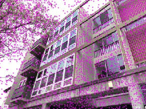
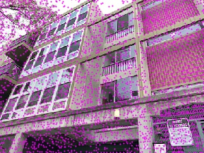
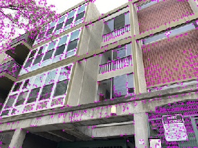
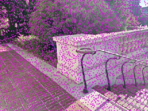
Part 1: Detecting Corner Features

I used the given starter code for Harris corner detection, to collect all of the Harris corners of each image and the corresponding corner strength. I also set a threshold value and filtered out corners with corner strength below this threshold. The Harris corners are shown on the following images. For each image, I first show the Harris corners overlaid on the image followed by the Harris corners on the same image with a threshold value.

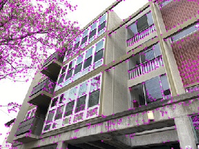
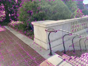
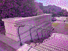
Part 2: Adaptive Non-Maximal Suppression

Continuing on from the corners identified in the previous part, I used adaptive non-maximal suppression as described in the paper to further narrow down the set of corners so that the remaining corners are all spaced a part from each other. I used the formula from the paper as seen below to calculate the minimal radius from each point to any other point and filtered down to the 500 points with the largest radii.

Part 3: Feature Descriptor Extraction

Now that I have 500 corner points for each image, I match the features between 2 images. I first define a window of 40x40 pixels around each corner and then downsample this to a 8x8 window, which is the descriptor for this corner feature. I also make sure to normalize the descriptor such that the mean is 0 and standard deviation is 1. I compare each descriptor in image 1 to each descriptor in image 2, and calculate the 1-NN and 2-NN as described in the paper, which are the two closest feature descriptors with smallest error between the descriptors. I only keep the feature pairs matched by smallest 1-NN is the ratio between 1-NN and 2-NN is below an error bound of 0.675 which I found from looking at figure 6b) in the paper. I show an example descriptor along with the sets of images and their feature corners.

Part 4: Robust Method (RANSAC)

After finding the matching features between the two images, I used RANSAC as described in lecture and the paper to compute the best set of points and the homography for these points by finding the homography that resulted in the most inliers. Inliers are the opposite of outliers and follow the homography correctly. I did a loop of 10,000 steps where for each step, I sample four random points and compute the homography. I then use this homography on all other points, and keep track of how many inliers there are for each set of four points where I define inliers to be when the distance between the homography applied on the point is within 10 pixels of the corresponding points in the second image. The final homography computed from RANSAC is the homography that contained the most inliers. At the end, I only keep the set of inliers as my final correspondence points.

Part 5: Final Manual and Automatic Mosaics

Now that I had the final set of corresponding points for my mosaics found from the methods above and computed the homography for these points, I created the mosaics with some blending as I did in project 4A. I have the manual and automatic mosaics side-by-side. In general, it seems that the automatic mosaics are slightly less blurry, although occasionally things in the foreground are slightly more in focus compared to things in the background.