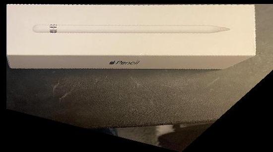
I used the following images for the sample rectification.
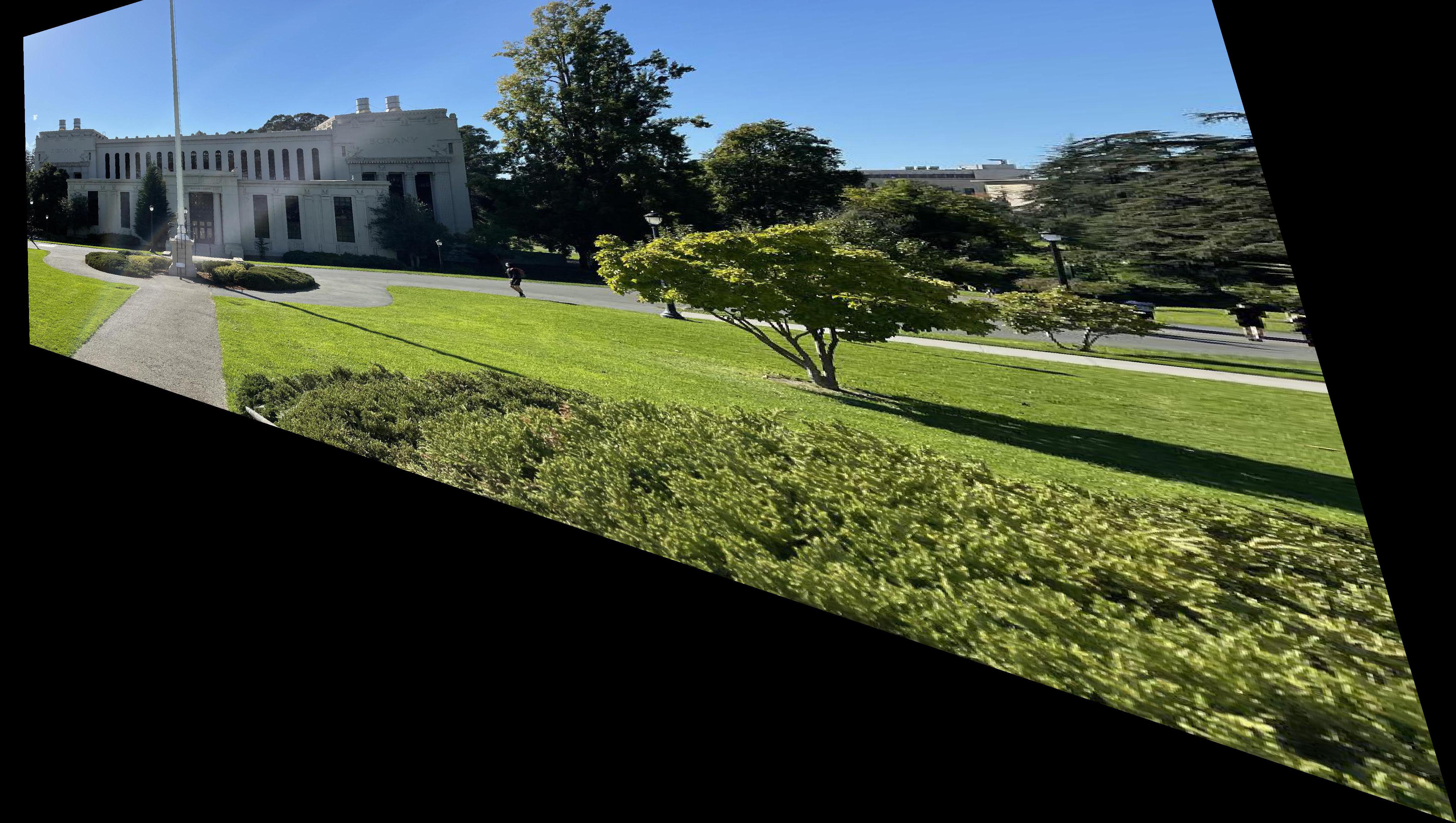
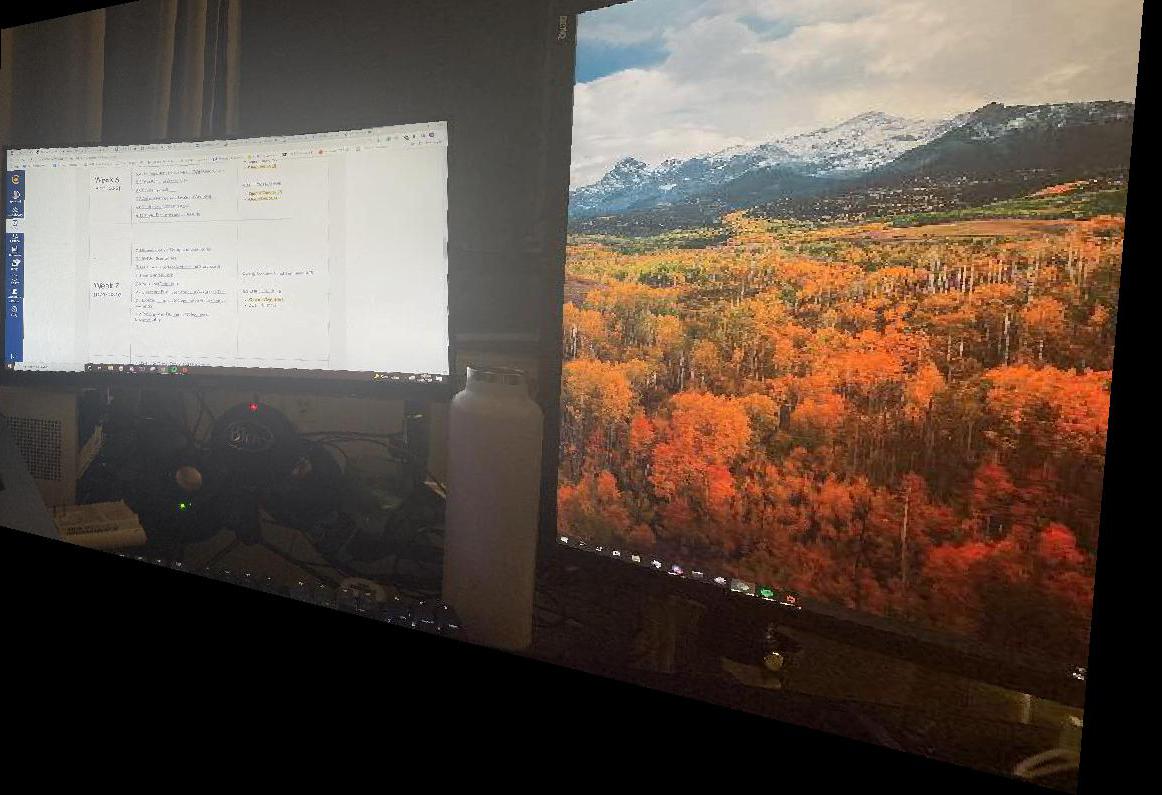
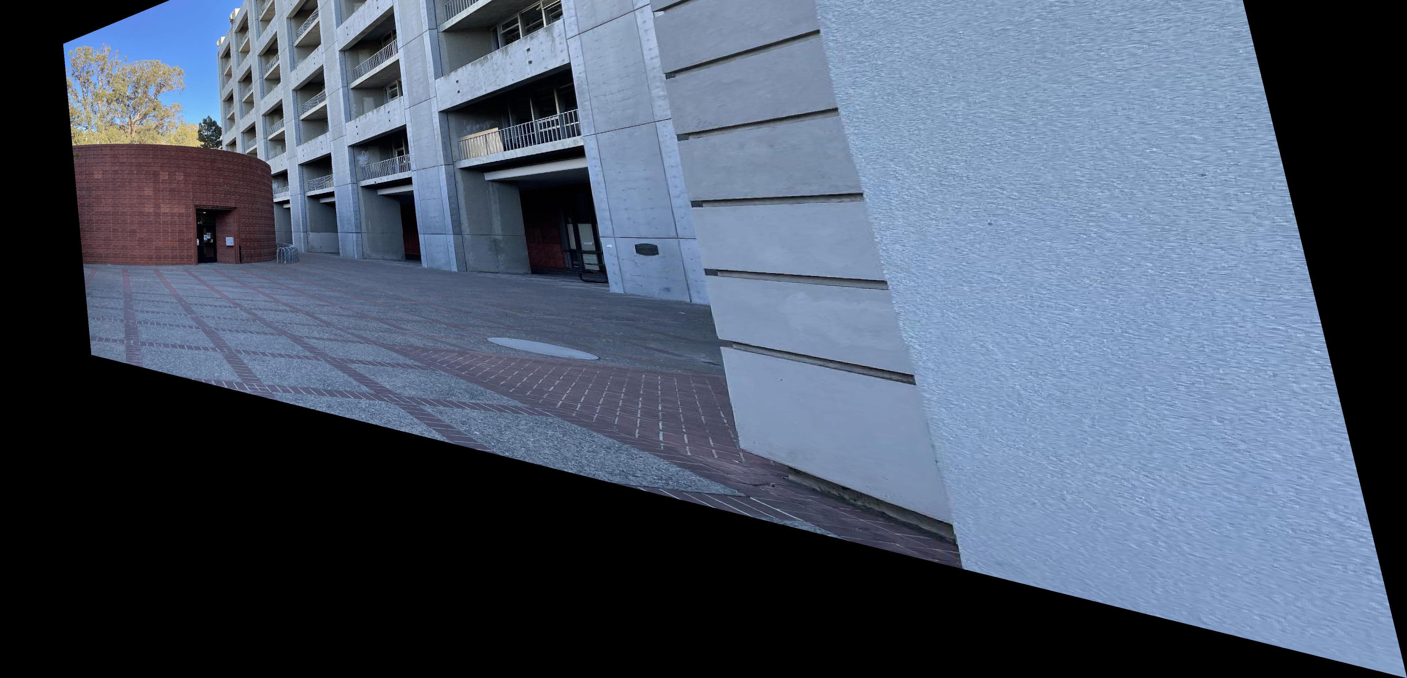
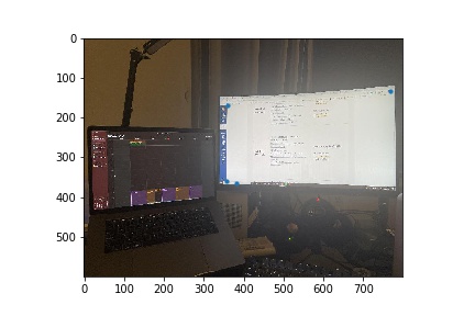
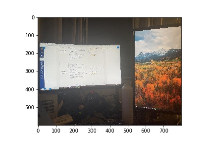
I used the following images for the mosaics.
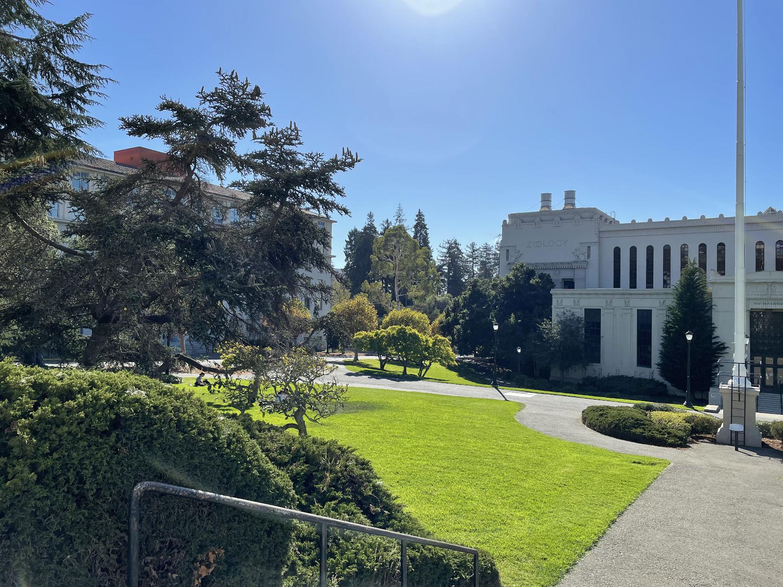
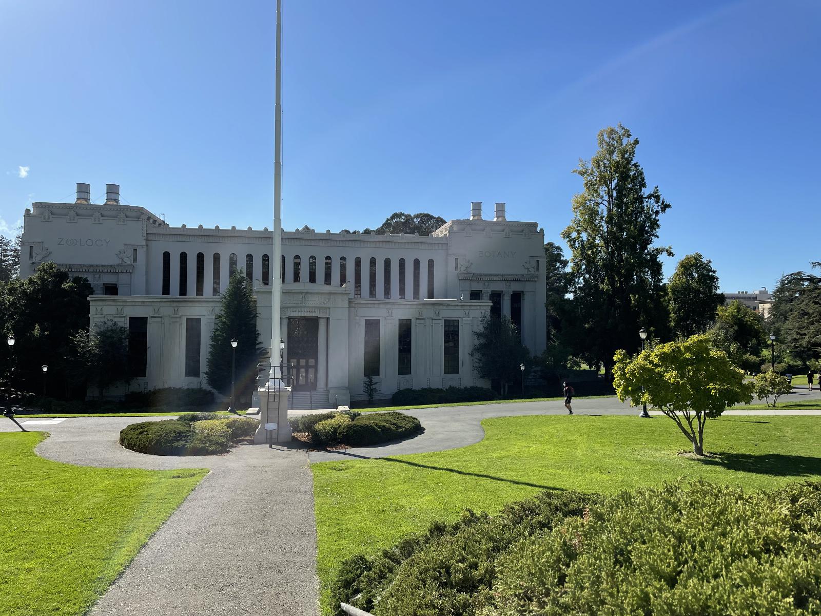
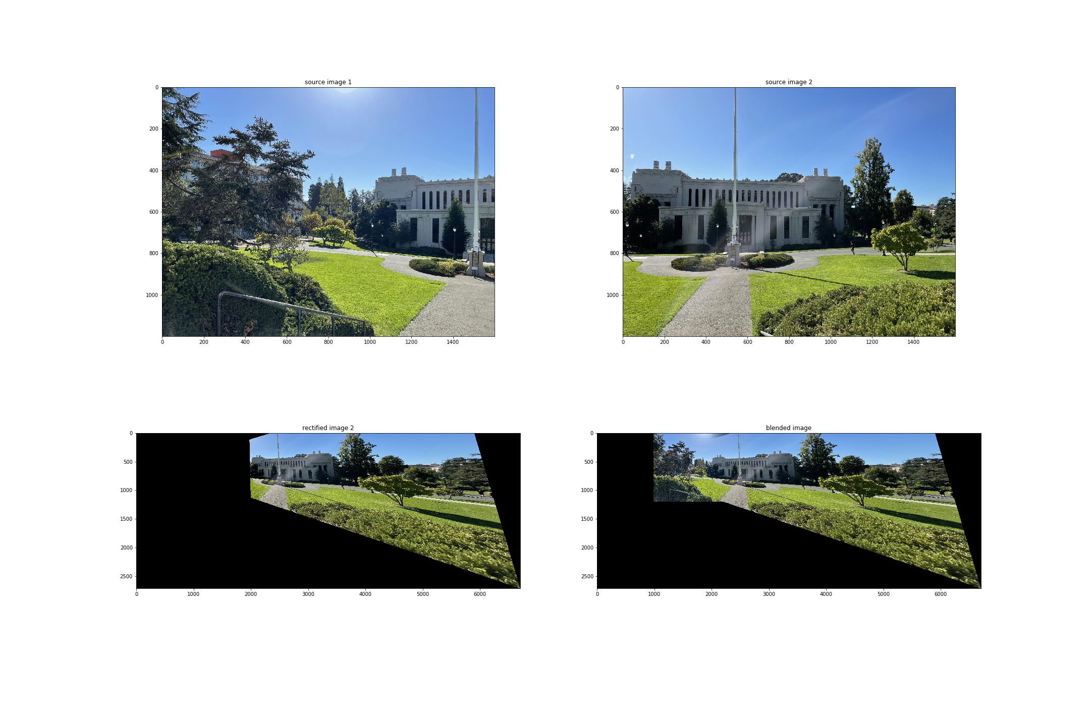
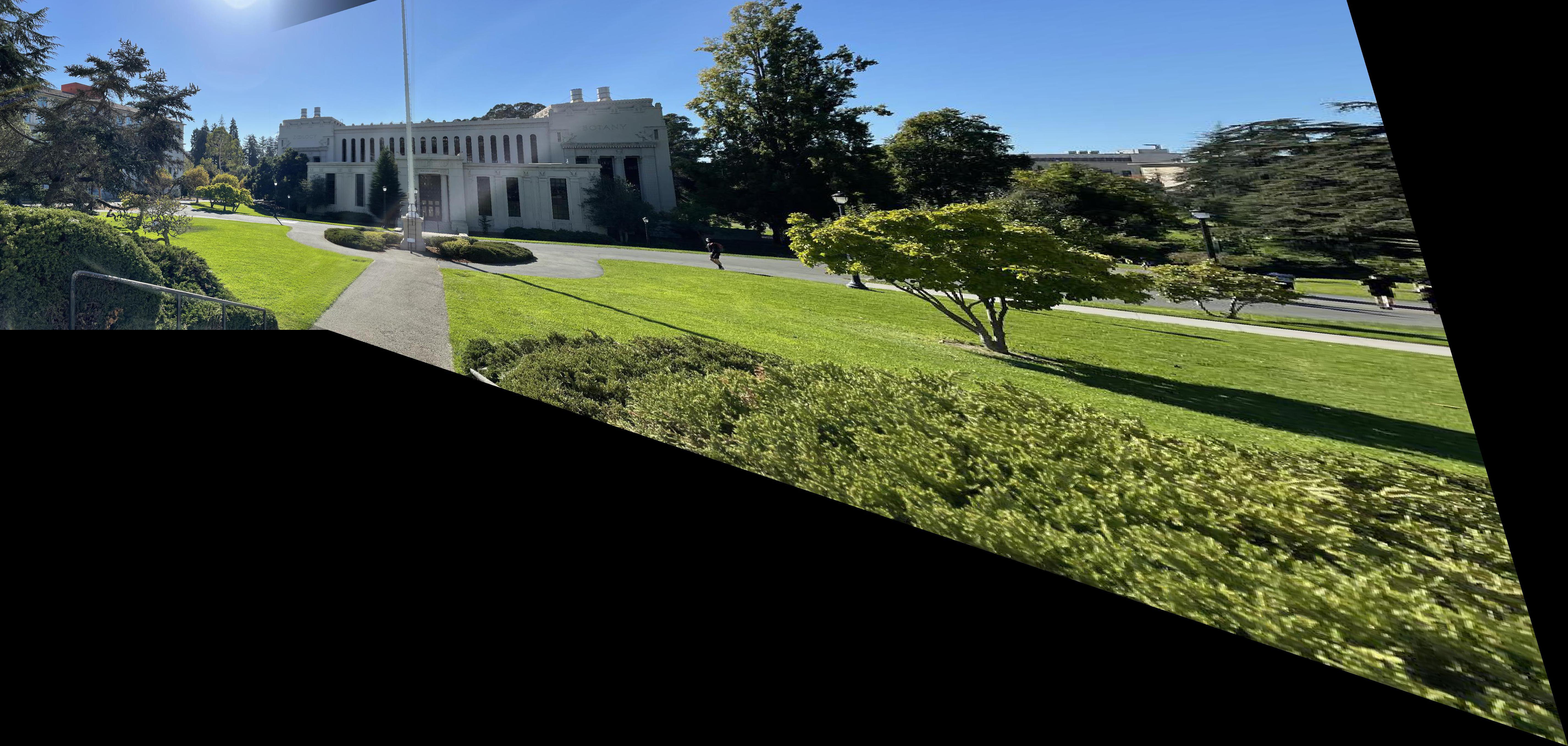
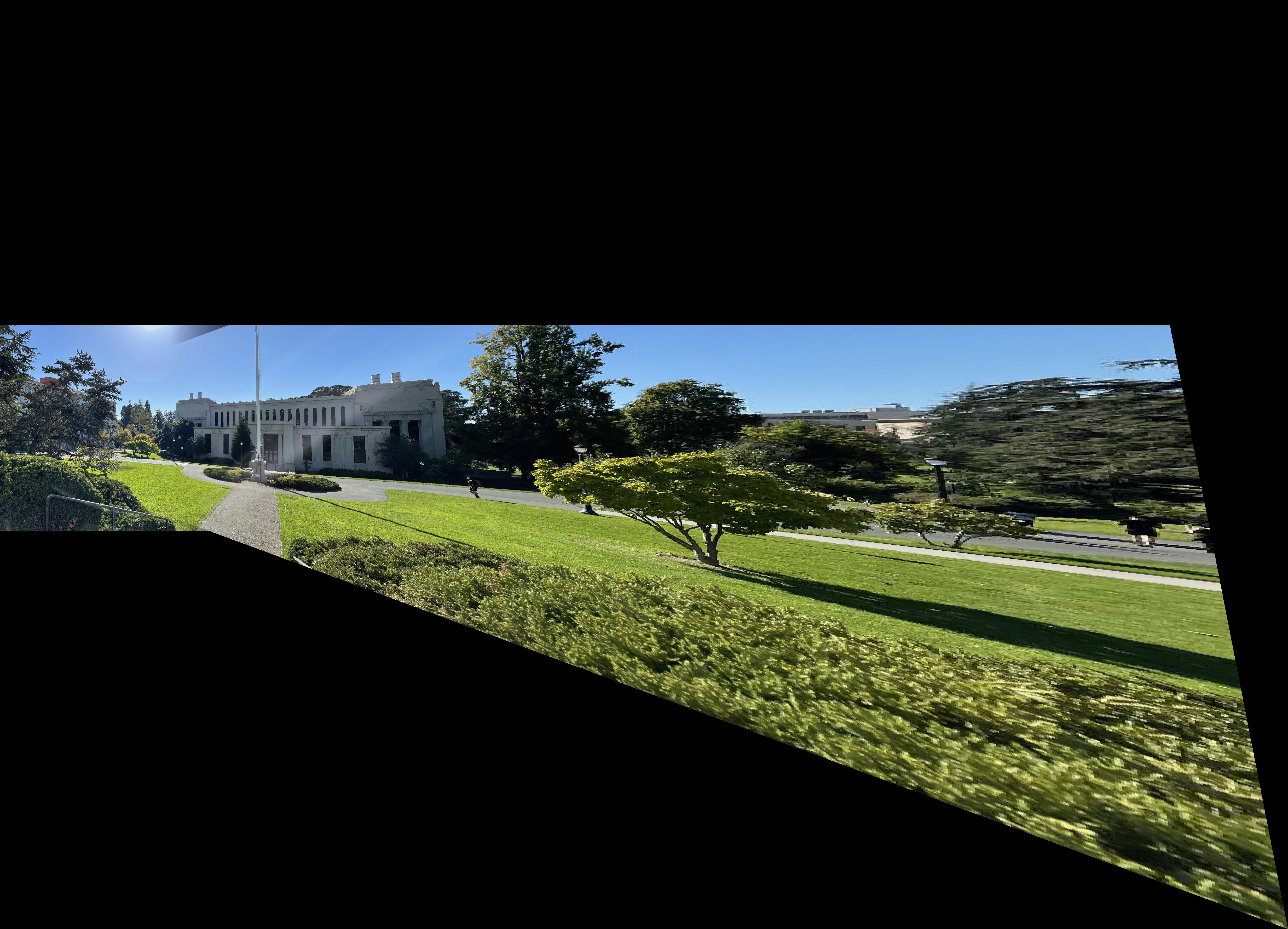
VLSB:
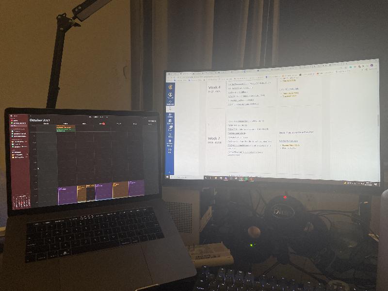
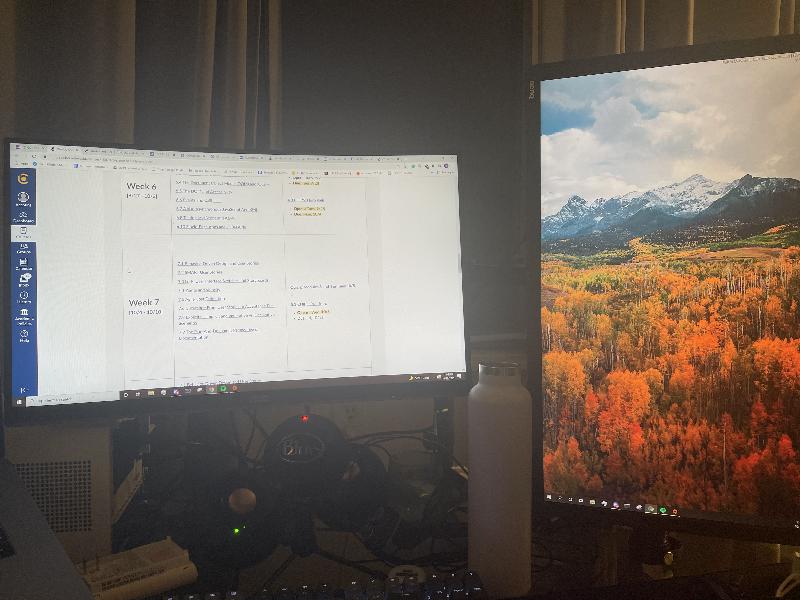
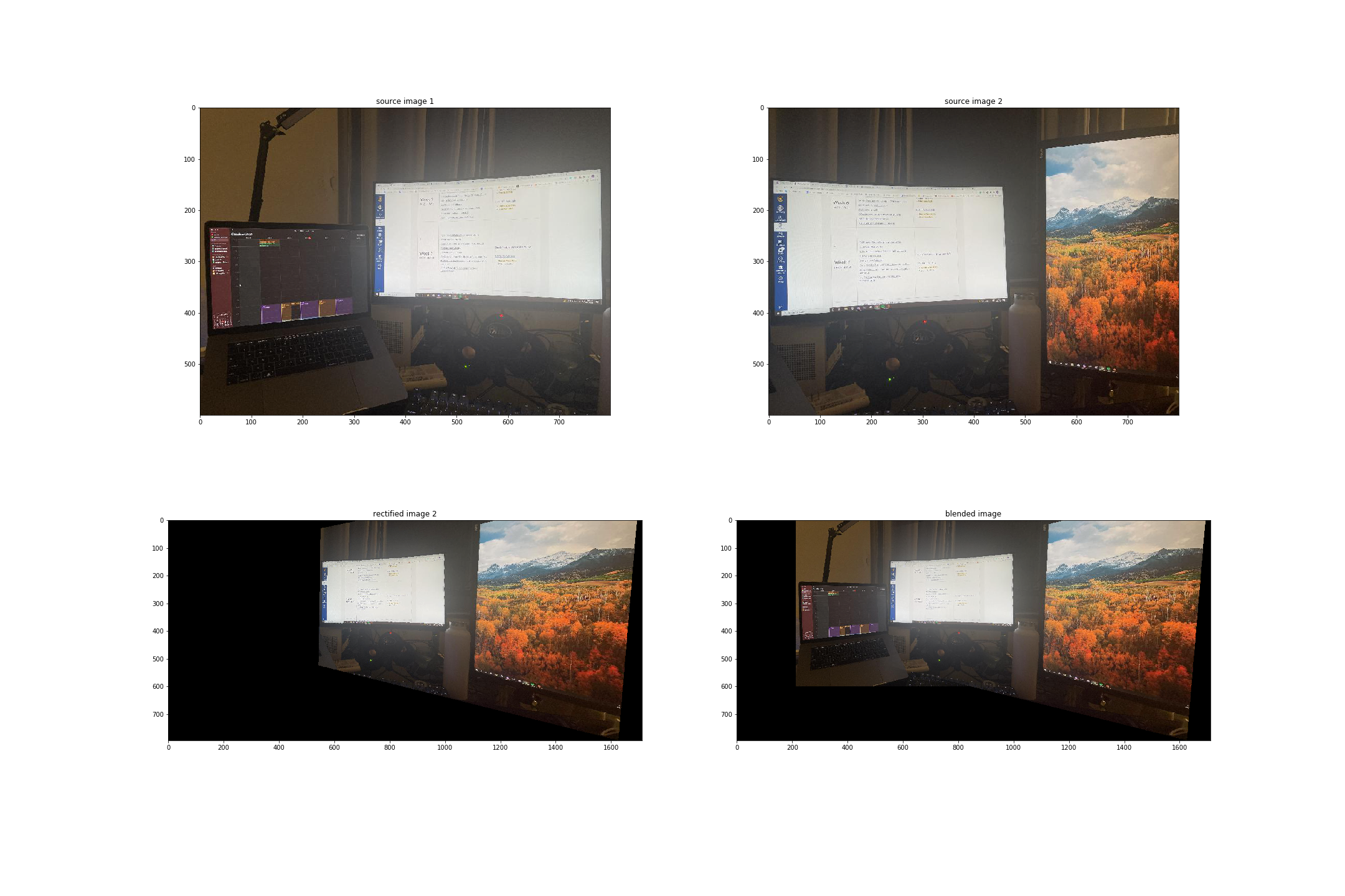
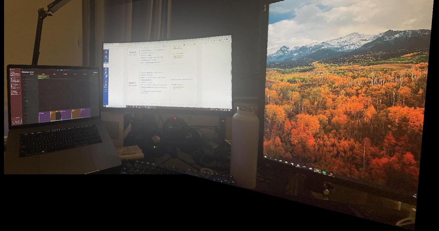
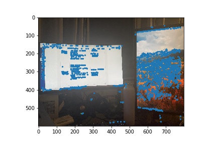
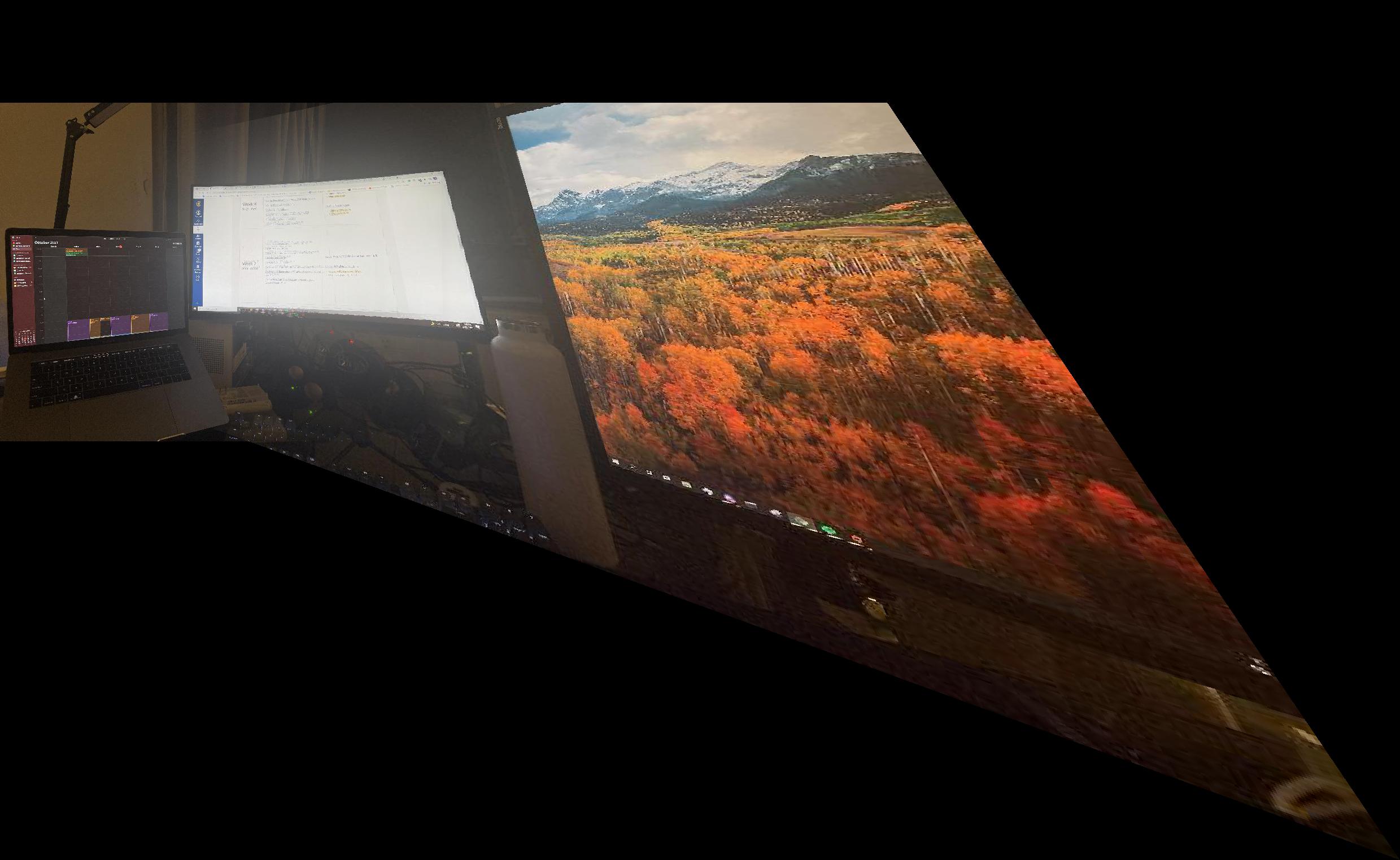
Monitors:
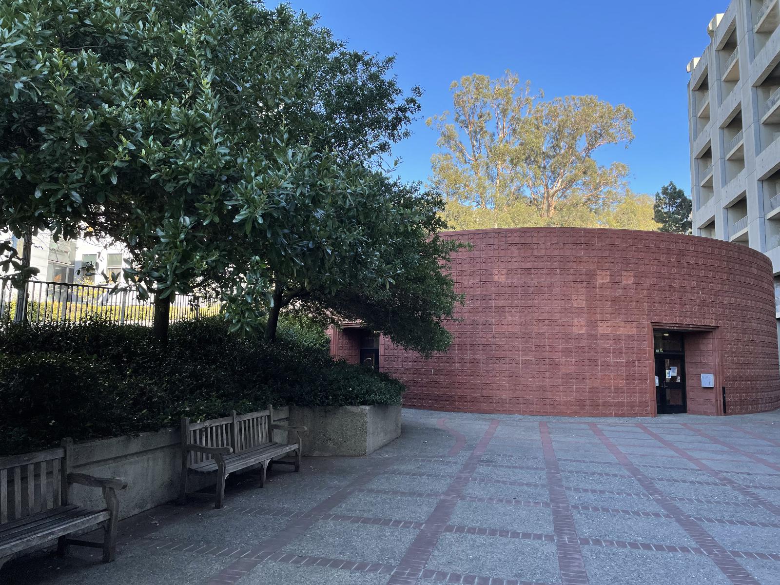
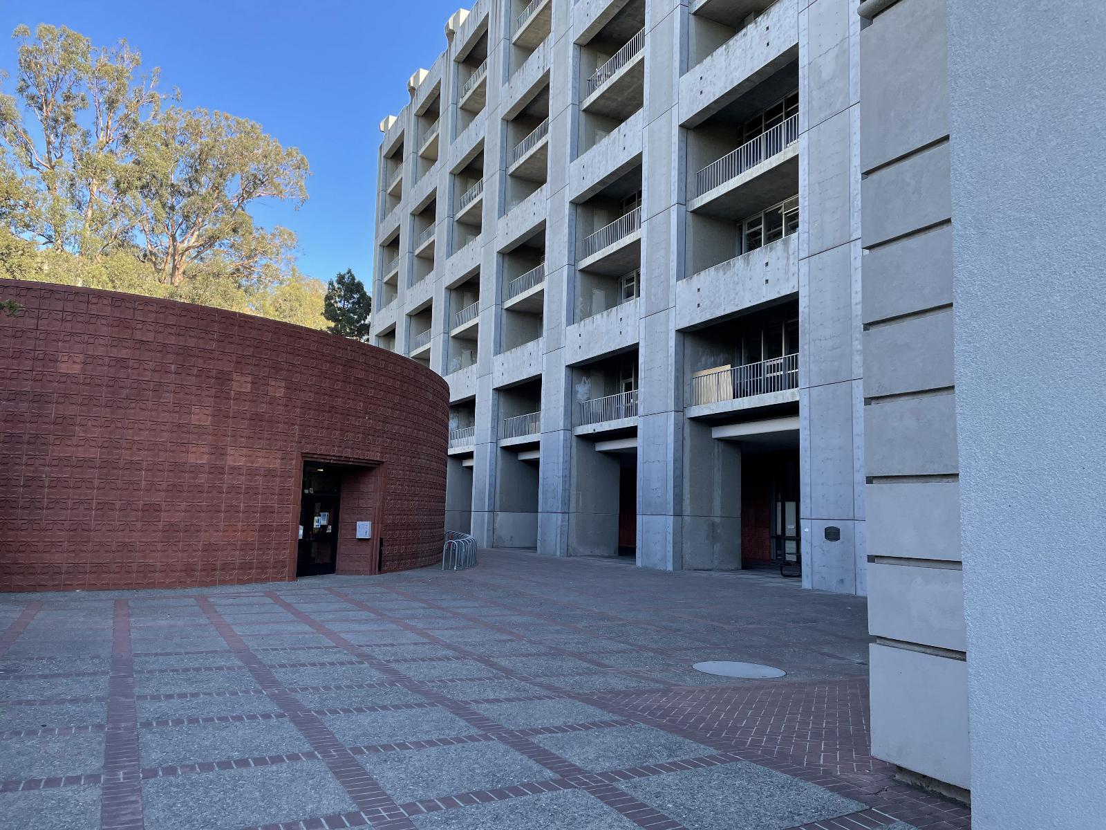
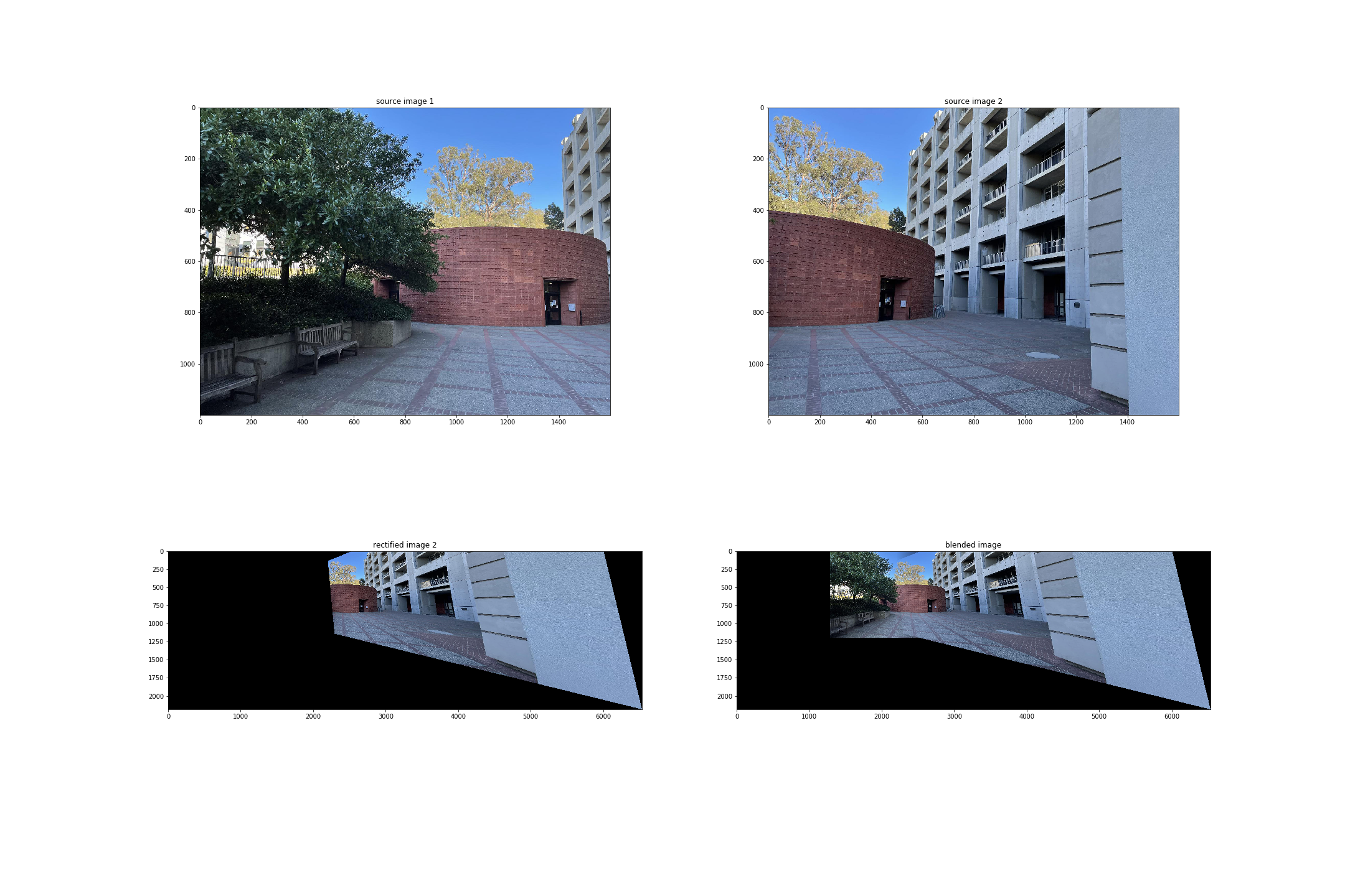
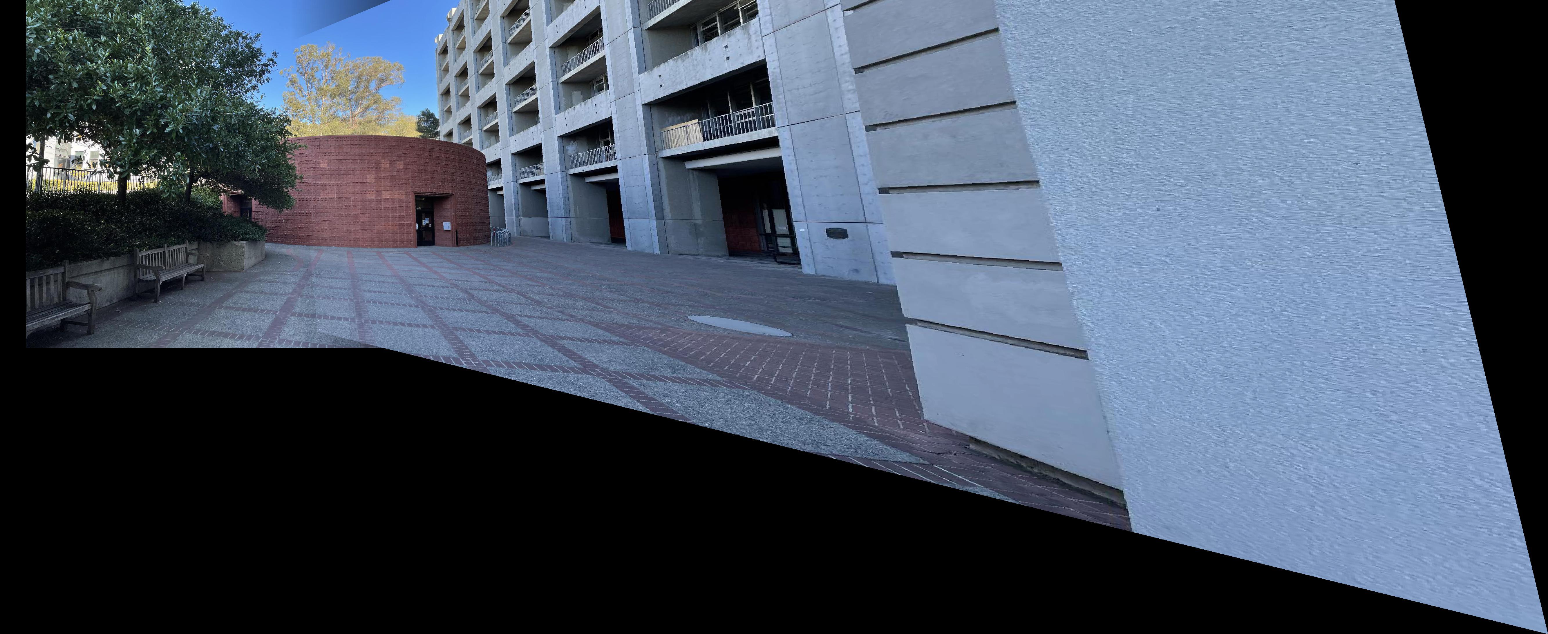
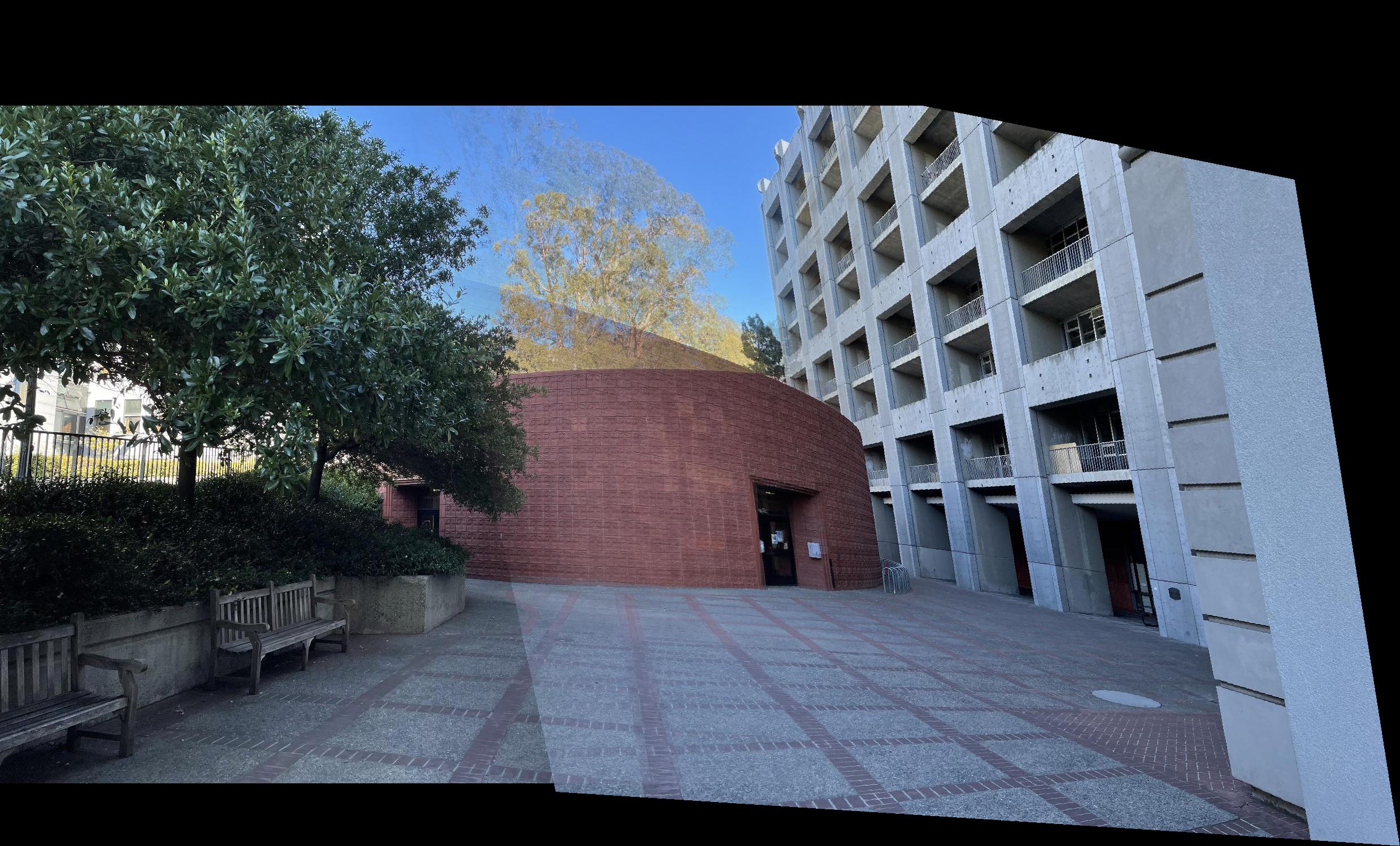
Pimentel Hall:
I recovered homographies by using the following equation reformatted so I could use least squares:
[w * x_prime, w * y_prime, w] = [a b c, d e f, g h 1] * [x, y, 1]
To get the values of the H matrix, for each coordinate in the correspondences, where x_prime, y_prime are the points of the source image and x, y are the points of the target image, we move around the system of equations and arrive at:
[x y 1 0 0 0 -x*x_prime -y*x_prime, 0 0 0 x y 1 -x*y_prime -y*y_prime] * [a b c d e f g h].T = [x_prime y_prime].T. We plug this into the least squares equation that minimizes the L2Norm of ||b - Ax||, where x is the flattened H matrix./p>
Warping involved piping the corners of image through H to get the boundaries of the mosaic. I made sure to get the accurate corners by dividing by the w value for each coordinate. I then populated the warped image with inv(H) * all coordinates defined by the polygon function using the new corners. Since there is mapping outside of the boundaries of the source image, I made sure to neglect those coordinates when populating (otherwise the boundaries are repeated). I also set up my warping function such that it would be easier to add the source image to when blending.
Below are my mosaic rectifications:
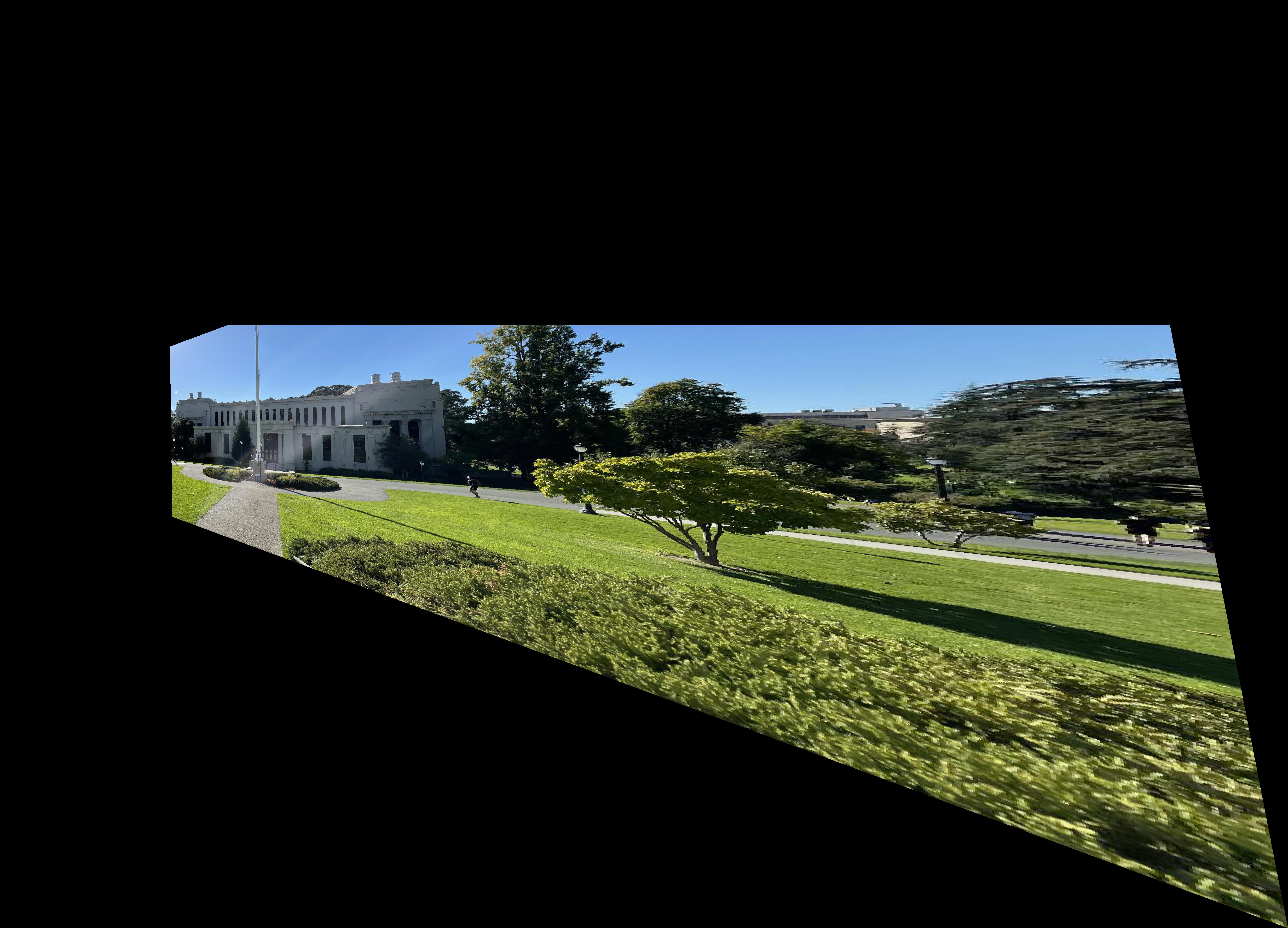
VLSB:
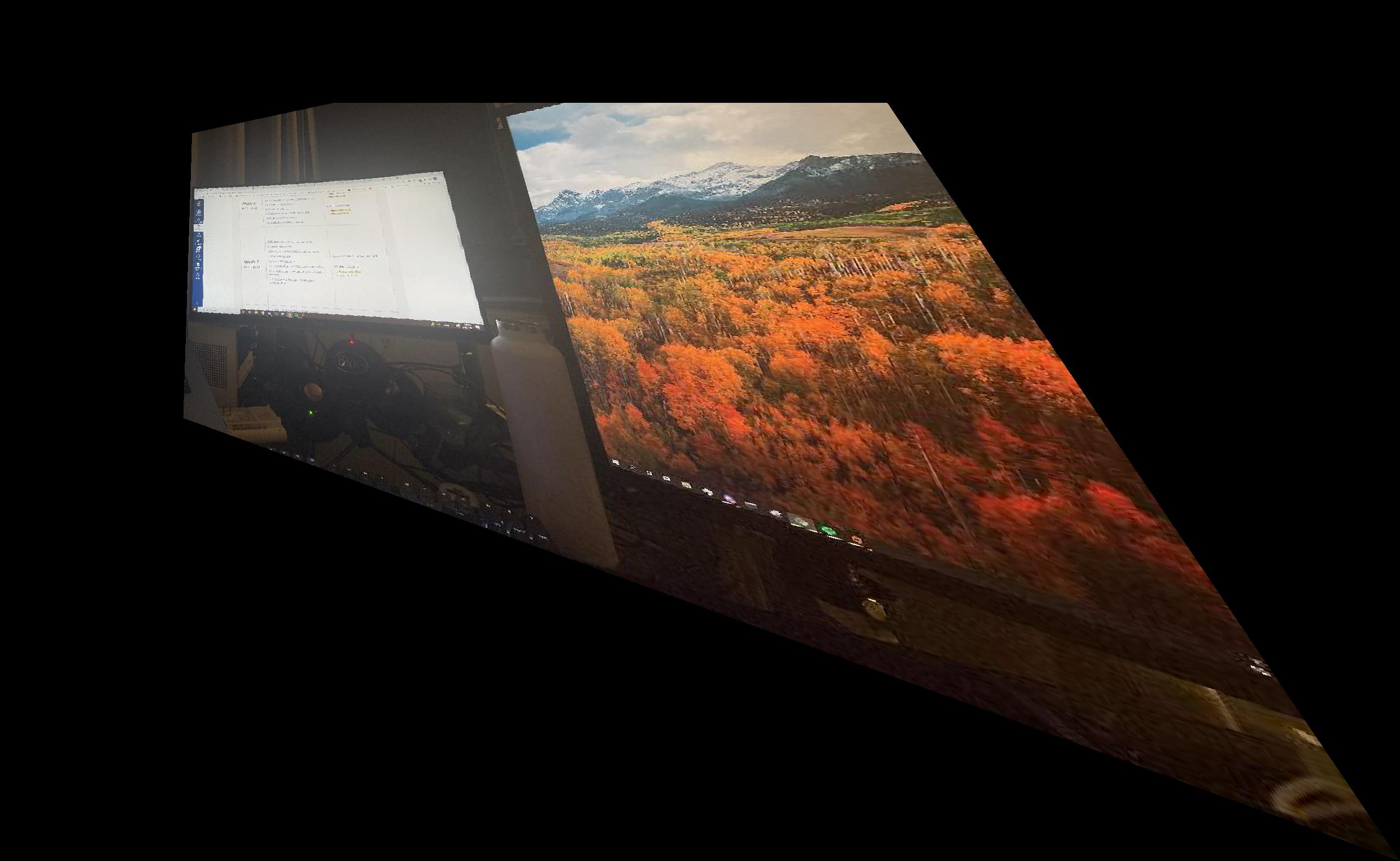
Monitors:
Pimentel Hall:
Below are my sample rectifications:
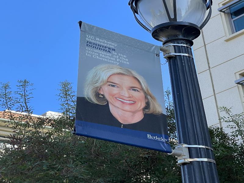
Jennifer Doudna:

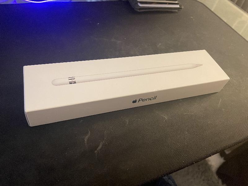
Apple Pencil:
My blending algorithm keeps both images at full capacity for non-overlapping regions, and holds alpha banding for the overlapping regions, this smooths the overlapping region & the troublesome edges. The results of my mosaics are below with steps.
VLSB:
Monitors:
Pimentel Hall:
I learned that it is incredibly difficult to achieve good or even decent results when manually picking out the corresponding edges. I also found great difficulty with warping, as I needed to make sure there were no index errors when projecting. I also learned firsthand the capabilities of linear algebra in image processing, and how we can map projections through recovering homographies.
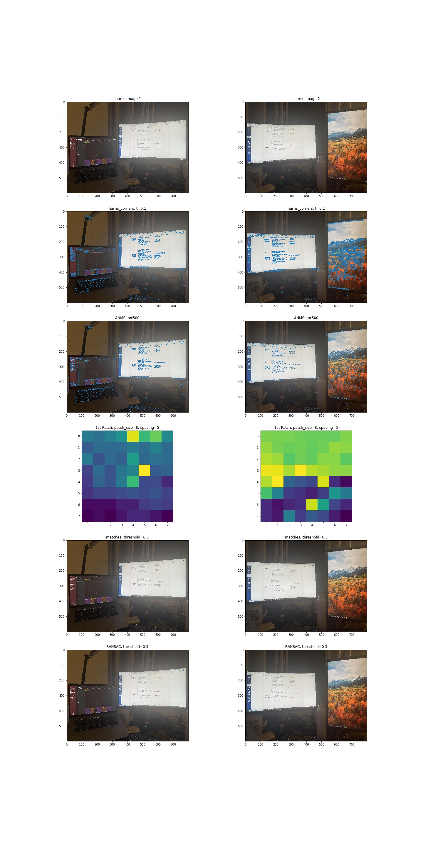
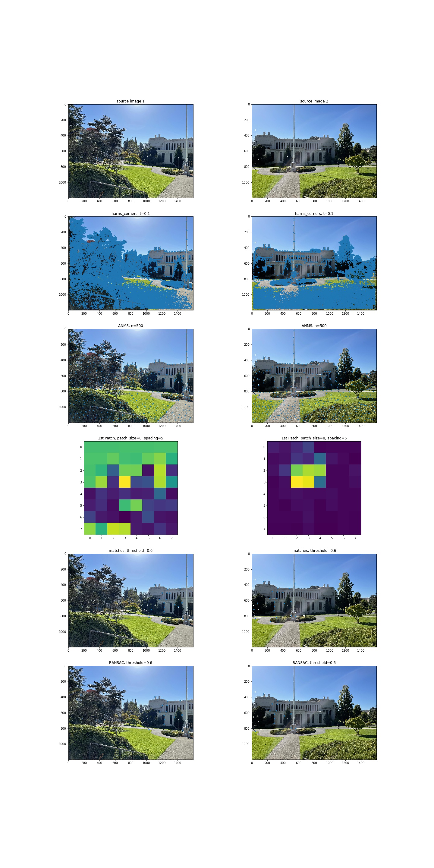
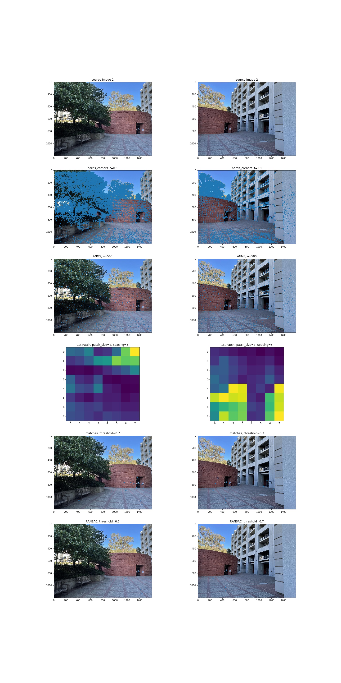
For finding Harris Corners, I used the starter code with an additional parameter of threshold_abs=0.1 in the peak_local_max method. Below are my monitor harris corners:
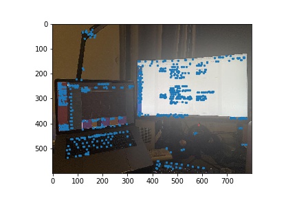
Using the ANMS formula described in the spec, I used c_robust=0.9 and kept the top 500 points with the largest radius. Below are my monitor ANMS chosen points:
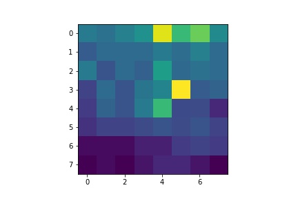
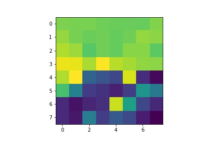
Using the Feature Descriptor described in the spec, I used 40x40 patches downsampled to 8x8 patches (window size=8, spacing=5). Below are the first monitor feature descriptor patches for reference:
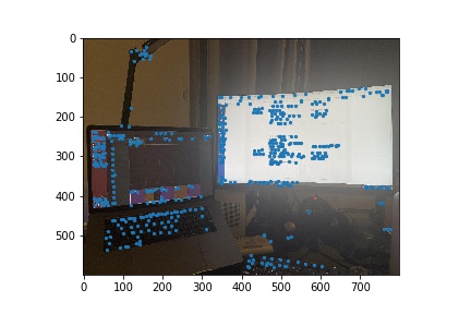
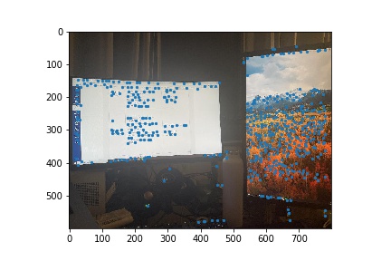
With the Feature Matching described in the spec, I used Lowe technique (1-NN/2-NN) with an initial threshold of 0.3 for my monitor mosaic, 0.6 for my vlsb mosaic, and 0.7 for my pimentel hall mosaic (These are captioned in the mosaics results section). Note that these are the only parameters I change between mosaics. I did this to ensure there were an adequate amount of points for RANSAC to iterate through. Below are the monitor feature matching points for reference:
With the RANSAC algorithm described in lecture, I used 10000 iterations with epsilon=10, as suggested, where each iteration I randomly choosen 4 points and compute the homography, then checking the distance between the transformed points and the complement points of the target image. I then found the points that satsified the epsilon threshold and updated the chosen inliers and chosen homography if the length was greater accordingly.


Here are the aforementioned steps in a comprehensive manner.
Here are my new rectified images for each mosaic.
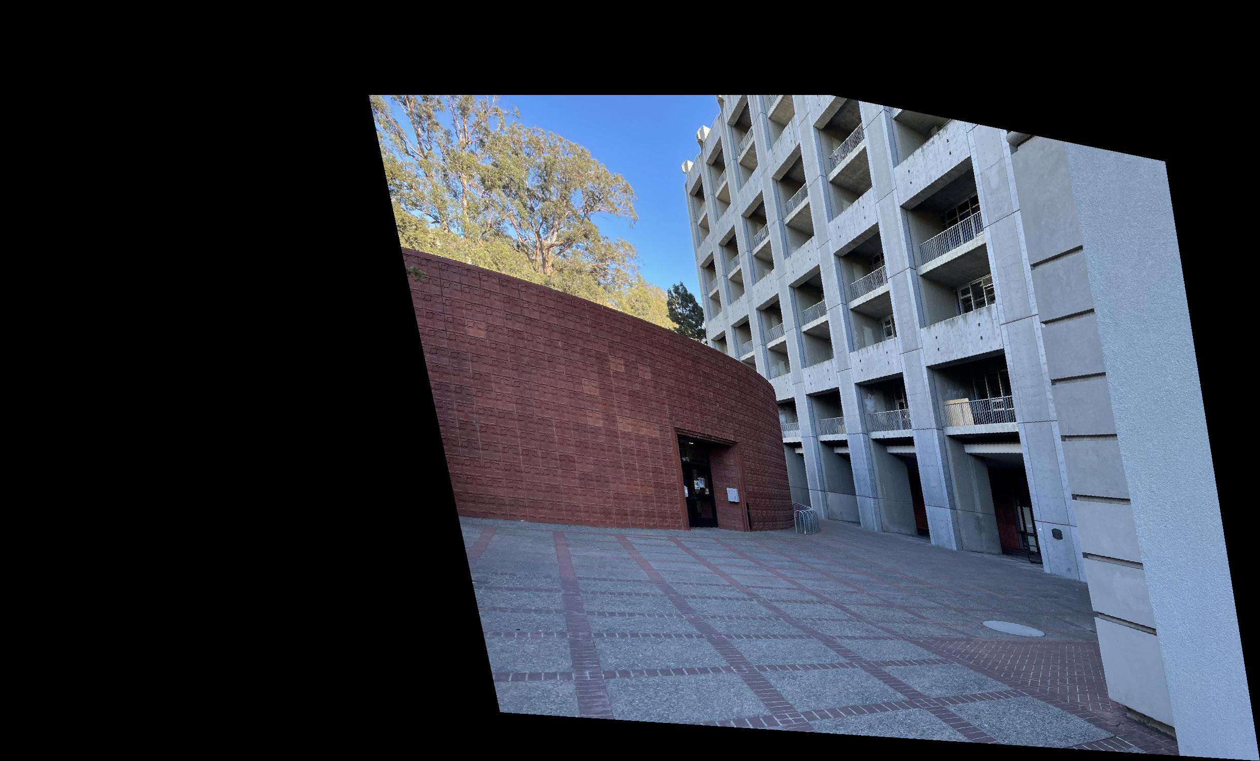
Here are my new autogenerated mosaics compared with the manual ones from Part 4A. Note that my pimentel mosaic performed worse, due to the improper angle from which I took my source image 2.
VLSB (Auto, Manual):
Monitors (Auto, Manual):
Pimentel Hall (Auto, Manual):
I associated image processing alot with machine learning before this class, so it was definitely interesting to see the mathematical side of associations used in this project, like RANSAC and feature matching with patches. It was also cool to put pseudocode and descriptions from a paper into practice.