Programming Project #4 (proj4A) (first part) (Ujjaini Mukhopadhyay)
Recover Homographies
To recover the homography, I solve a system of equations. I know that applying a homography warps an image so I can do somehting where p' = Hp where H is a 3x3 matrix. I know that the bottom right corner must be 1, so I have 8 degrees of freedom. I can solve this using 4 points since each point gives me two pieces of information, but it is better to solve this as a least squares problem. I first define correspondences on my images, and form a matrix that looks something like this:
Warp the Images
To warp the images, I take in my image that I want to warp and my calculated Homography. I want to do inverse warping so that there are no holes in my final object. Thus, I calculate the inverse of the homography, find all the points on my final image that I want to warp and remap them accordingly. I took a lot of inspiration from https://stackoverflow.com/questions/46520123/how-do-i-use-opencvs-remap-function and piazza.
Image Rectification
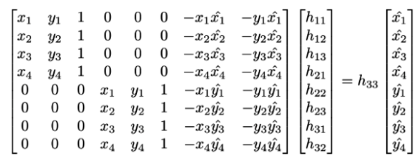
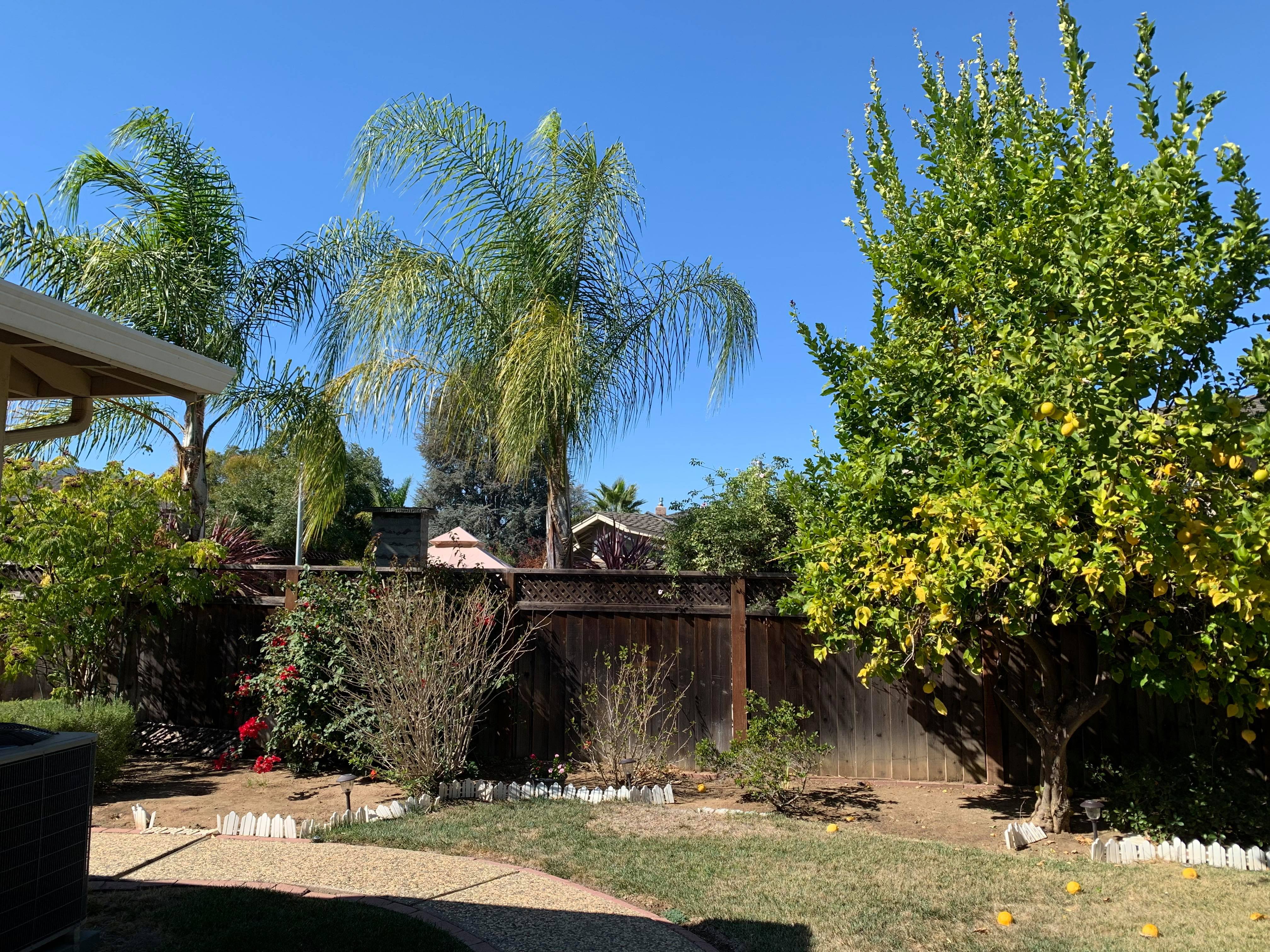
To show that my warping works, I rectified the following image to make it seem frontal parallel.
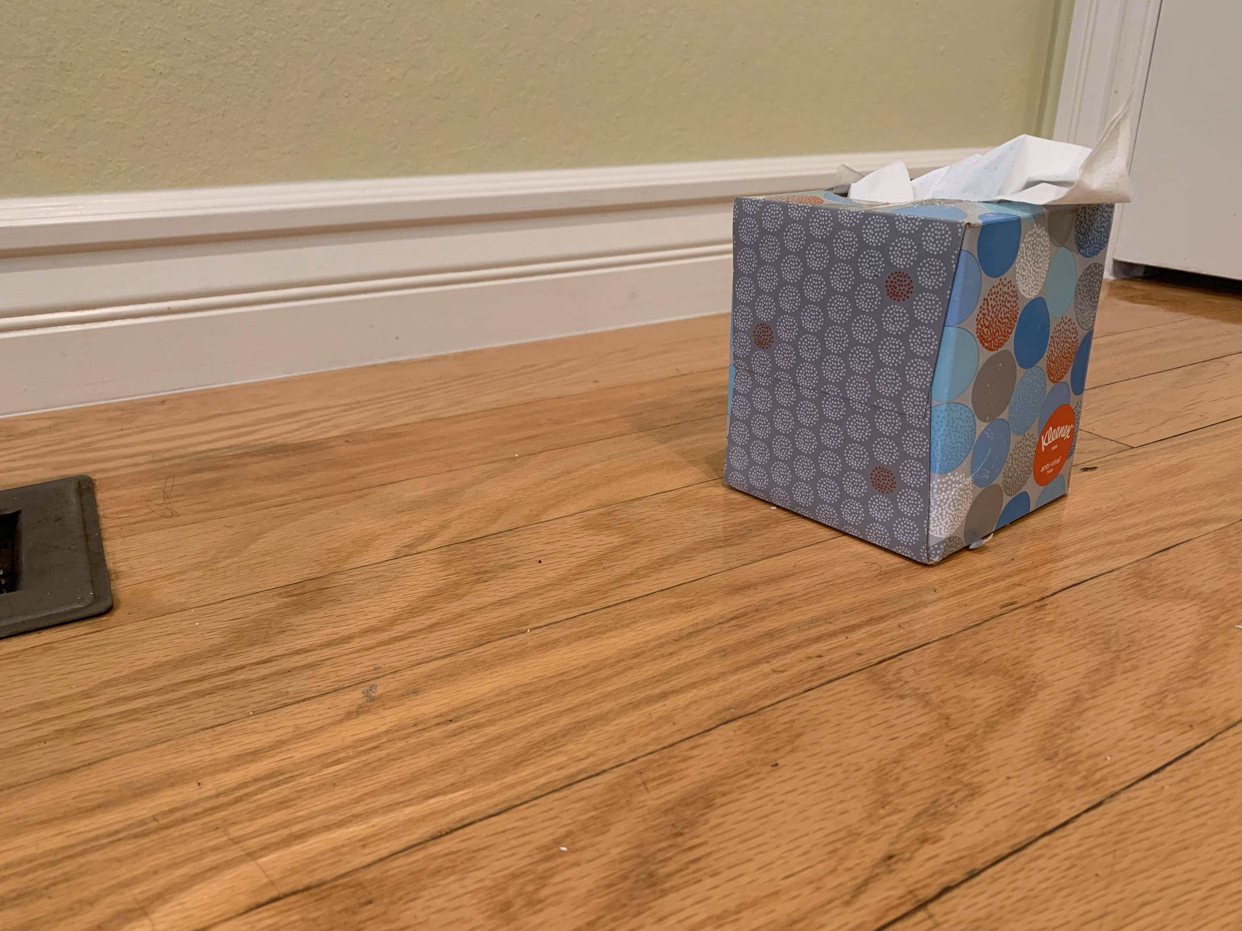
Here is the original image:
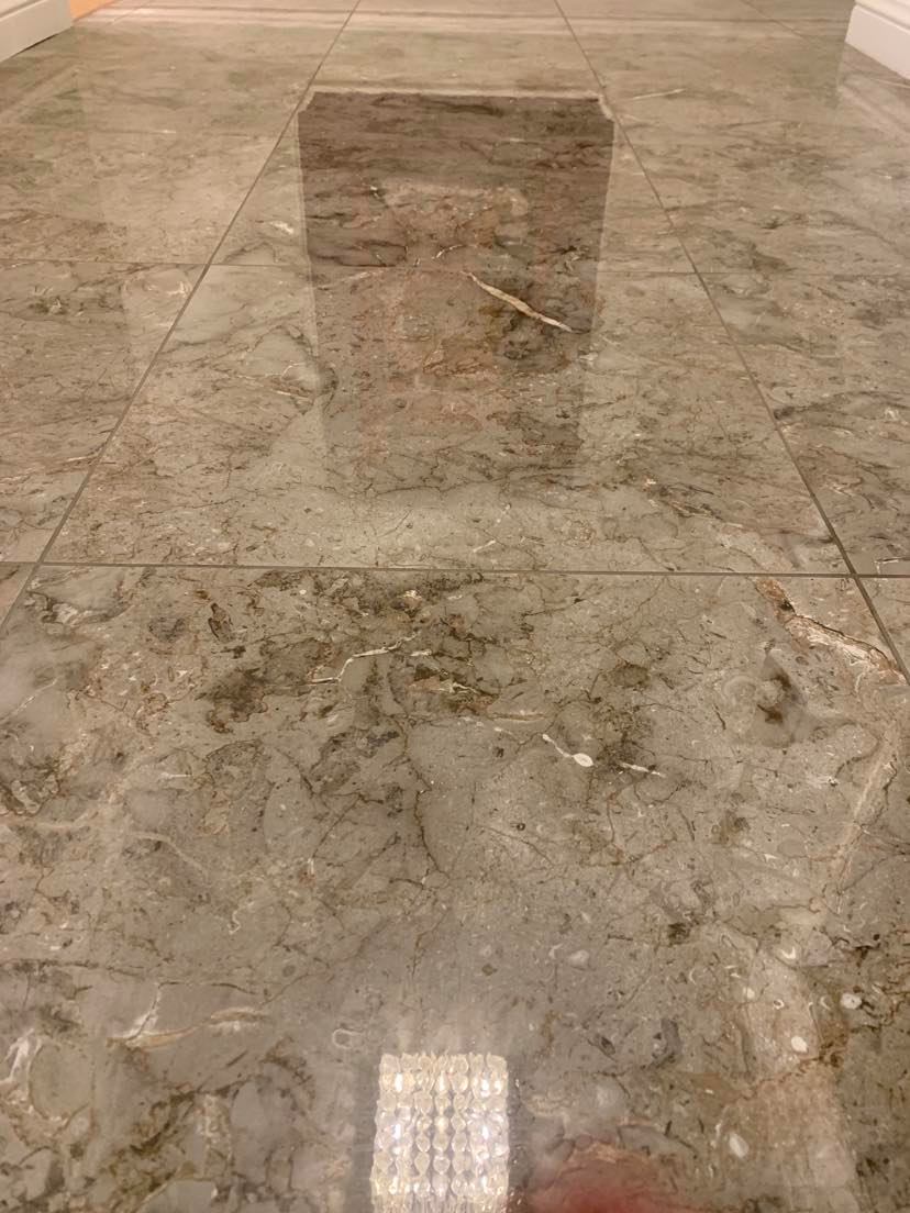
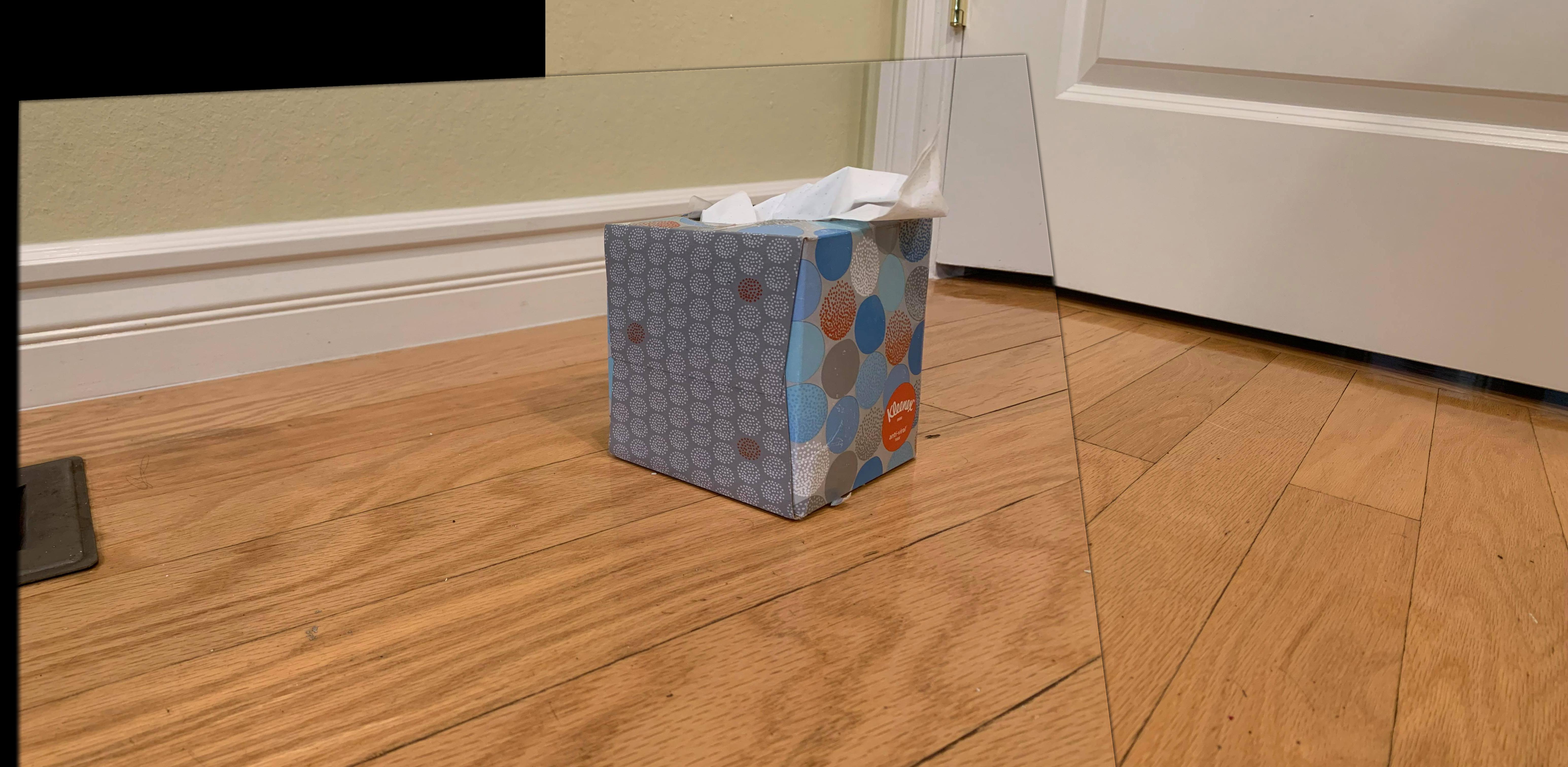
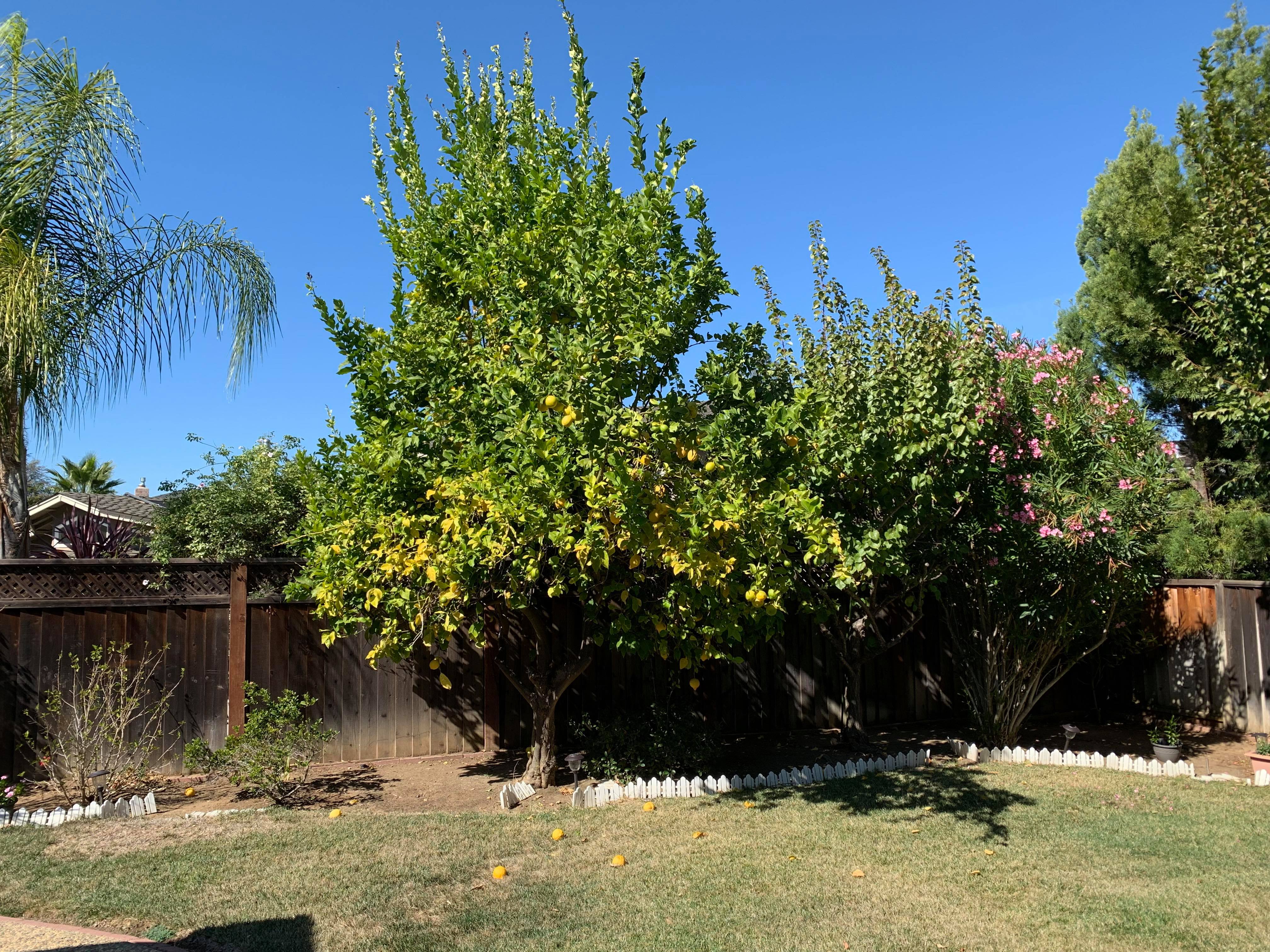
Here is the warped image after selecting four points and setting their final points to be square:
As you can see, this is the frontal parallel version. I also did the same with another image:
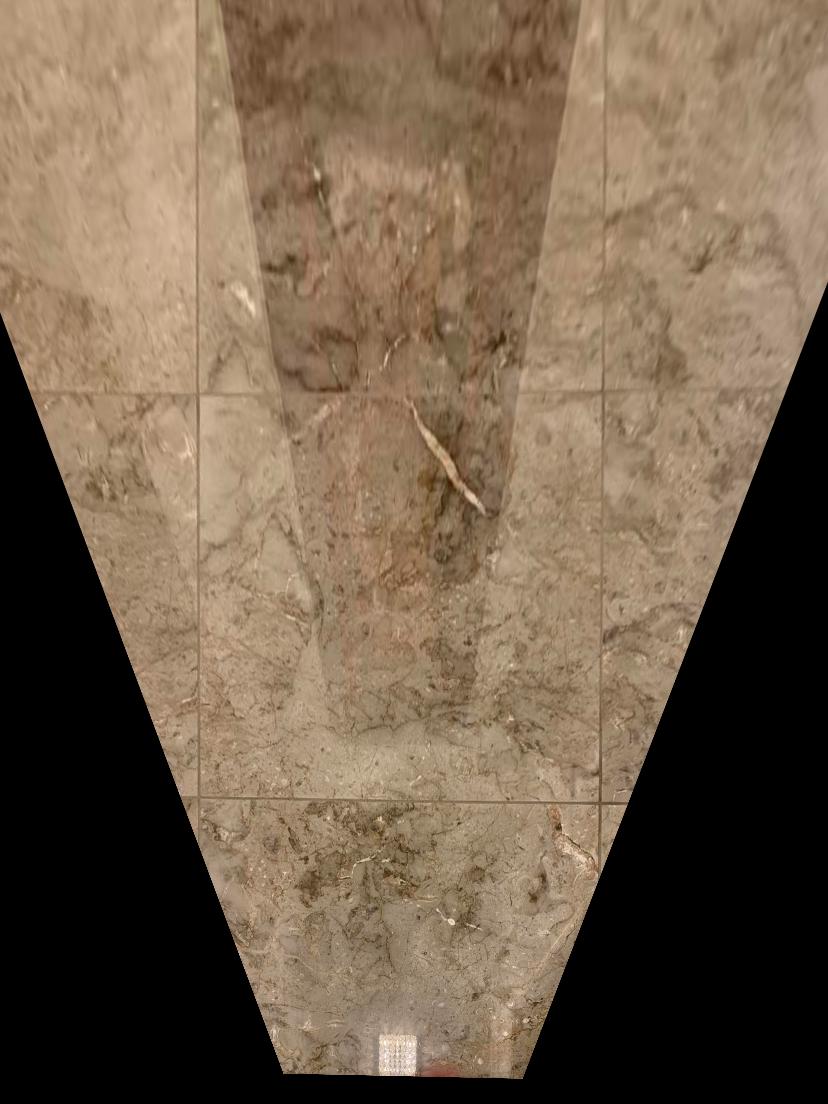
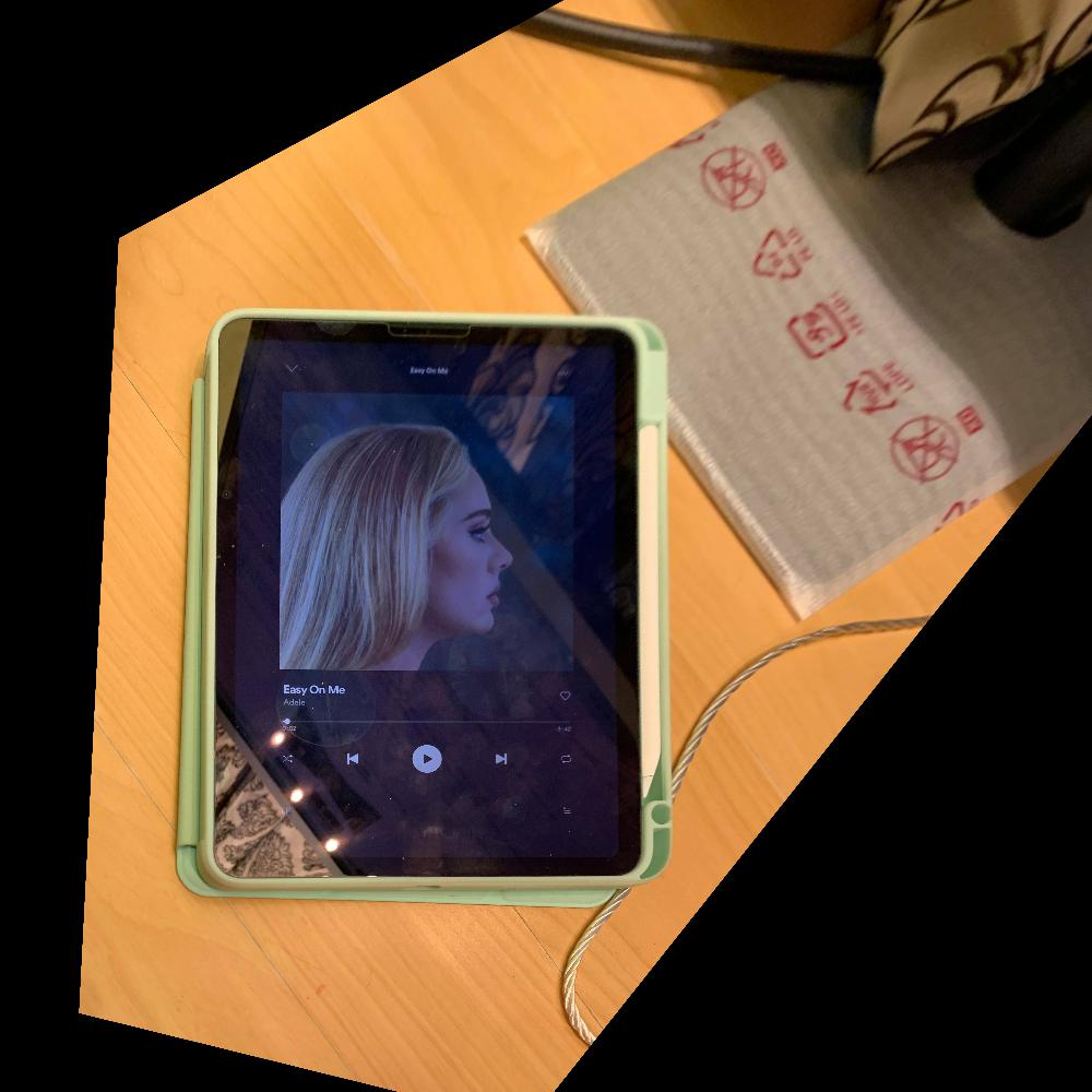
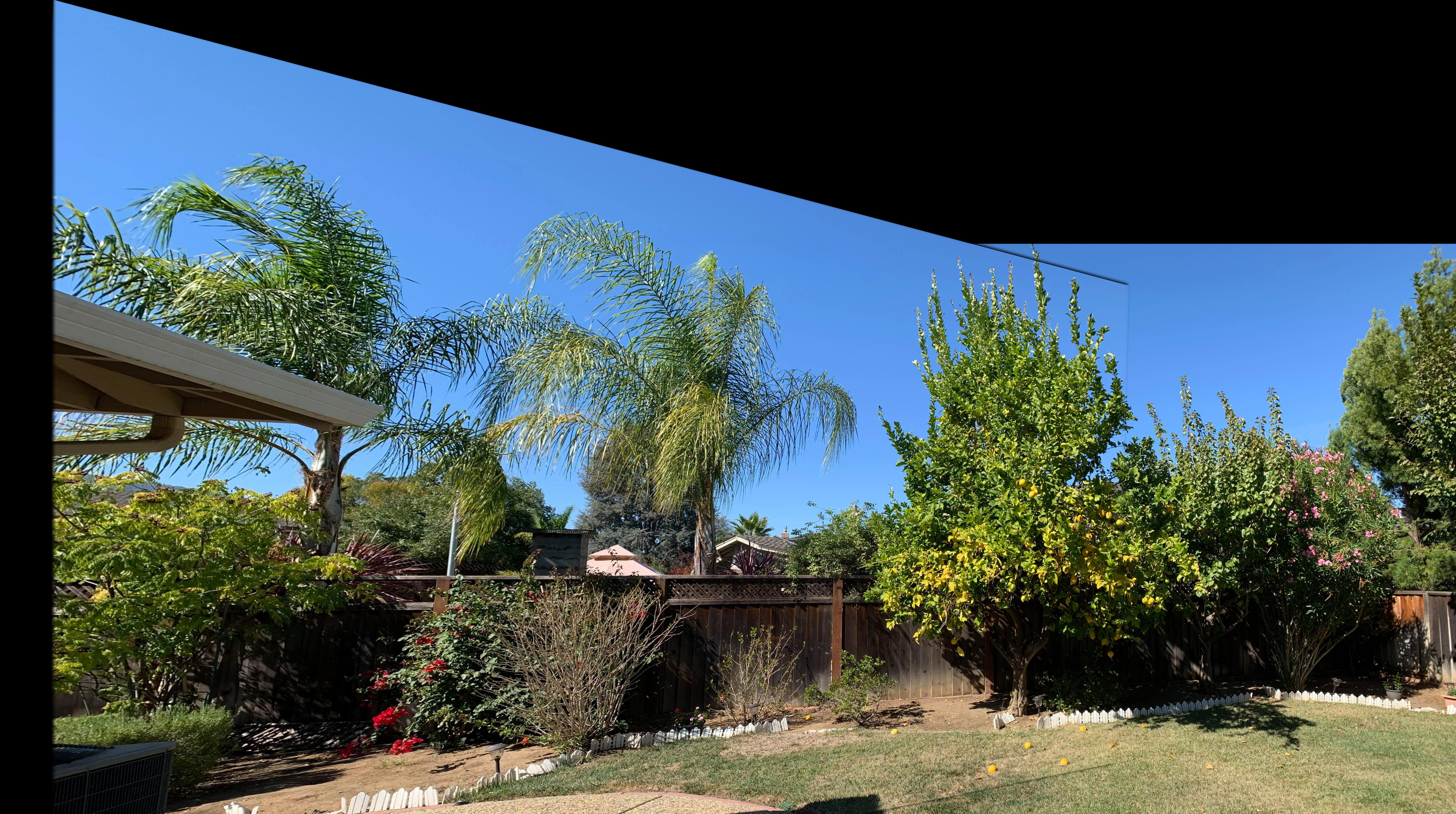
Here is the warped image after selecting four points and setting their final points to be rectangular (kind of in proportions of the iPad) -- also, Go Adele!:
Blend the images into a mosaic
Now that I can warp, I can build larger canvases, warp to them, and display panoramas. The method I chose is to constantly warp the left images and add in the right image as I go through a list. I was always calculating the corners and if any of the left corners were negative, I added an x_offset and if any of the y values were negative, a corresponding y_offset as well. For blending my seams, I used Gaussian Blending. To create the mask, I used polygon between my corners (brought the corners in a little bit so that the edges are less obvious) and created a gaussian stack.
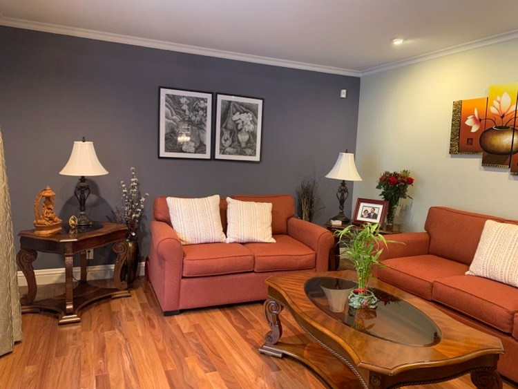
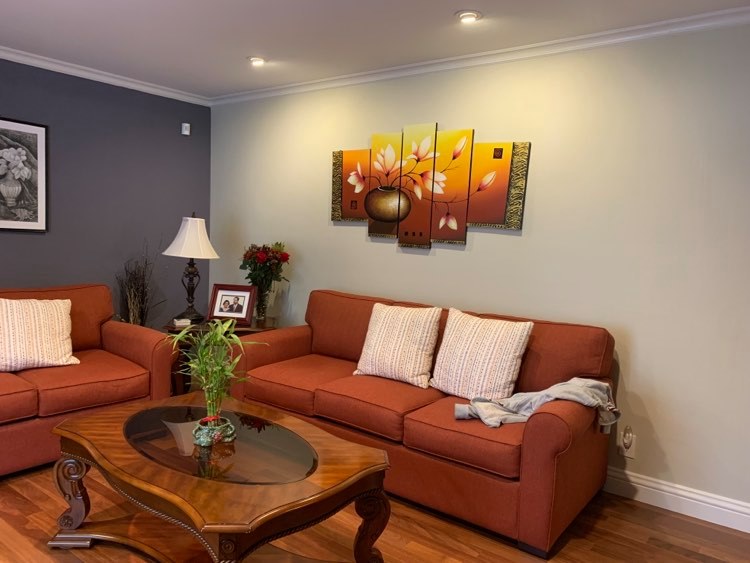
Here are some examples:
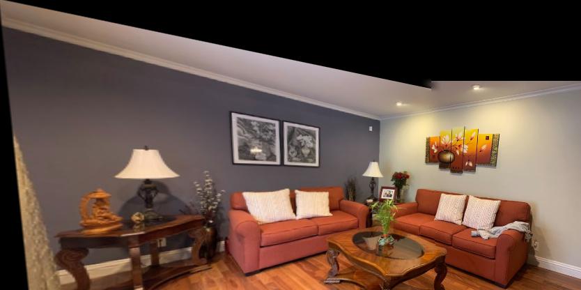
Adding on another photo, this is my final panorama:
Through this project, I learned the importance of defining correspondences correctly. I put together 3-4 more panoramas which all failed becuase the pixels weren't exact. Had I had more time, maybe I would have gone back to fix the correspondences. I tried variations of choosing 4 points, 10 points, even up to 30 points and used Least Squares solutions to solve, but even so, small mistakes or even un-compatible pictures made the panoramas very difficult to put together.
Programming Project #4 (proj4B) (second part) (Ujjaini Mukhopadhyay)
Harris Corners
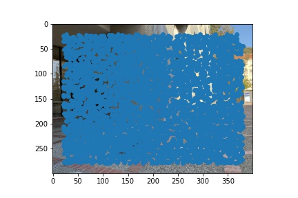
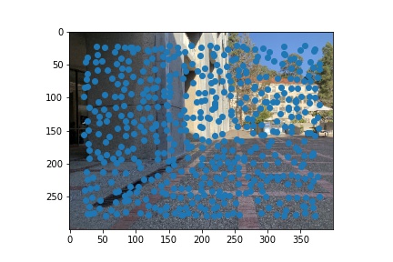
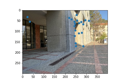
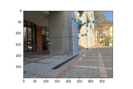
Harris corners work by looking at junctions between two edges (i.e. corners). Corners are important because they exist through all kinds of transformations (i.e. the optic flow issue covered in lecture). By only looking at corners we are able to drastically decrease the number of points we consider as matching for finding correspondences. Here are some examples of harris corners. Setting the threshold will help get rid of any points that are not corners. However, this reduces the number of possible matchings. In these images, the relative threshold is around 0.1. I set it this low because I knew that some points had very strong corner strengths but because of qualities in my image, 0.1 seemed to return a good, workable set of points. In the following pictures, you'll also notice that it seems that most of the picture is covered. HOWEVER, this is likely because of my blue dot's size.
Adaptive Non-Maximal Suppression
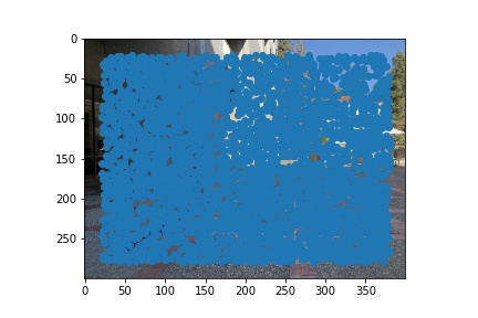
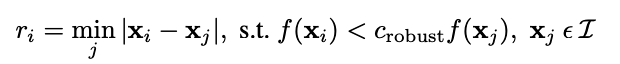
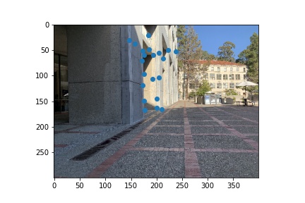
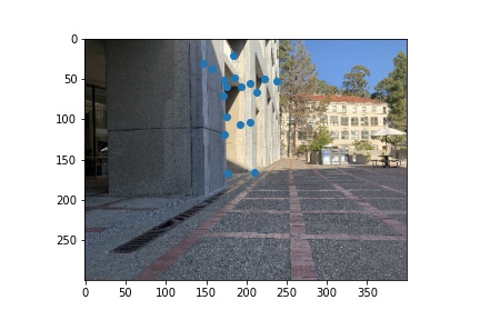
While corner strength is an important metric for identifying corners, it is possible that all corner points are clustered together in such a way that no set of points is overlapping. Comparing all Harris Corners above is also very inefficient so to reduce the size of the set and get a more even distribution, we use ANMS. Essentially, it takes the local maxes of corner strength. To implement ANMS, I first found the suppression radius for each point.
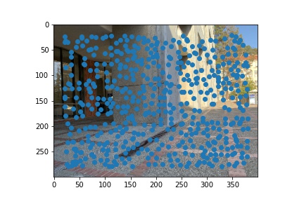
Then I sorted the coordinates by the suppression radius in decreasing order and returned the top n. Now I get the following images (in this example, I only got my top 50):
Feature Extraction Descriptor
To do feature extraction, for each point that I was returned from ANMS, I created a box that ranged from 20 pixels to the left to 20 pixels to the right, 20 pixels from top to 20 pixels from bottom to create a 40x40 box. Then I used cv2.resize() to make this an (8,8) patch. I then normalized all the numbers in the patch so that the mean is 0 and standard deviation is 1. Here is an example of a feature descriptor:
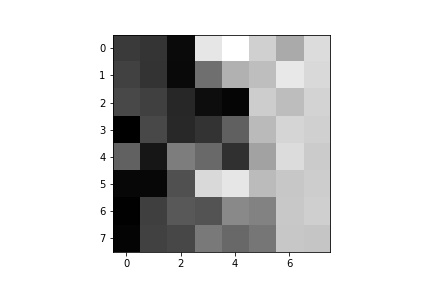
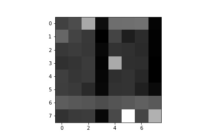
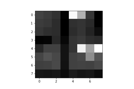
In reality, there is no aliasing because cv2.resize() uses some kind of blur. However, because I am displaying this image at much higher size, it looks like blocks.
Feature Matching
To match features, I simply took the ssd of their feature descriptors to compute nearest neighbors. After I got the first and second nearest neighbor, I took their ratio and compared it to a threshold. According to the paper, 0.33 was a good threshold that provided the least amount of error. In some of the panoramas to follow, I used an even smaller threshold to filter out more points that weren't perfectly matched. The idea here is that if the distance to the first neighbor is pretty close to the distance to the second neighbor, then it is likely that this pair of points is not a good matching. Here are some points that were matched:
Random Sample Consensus
Finally, I implemented RANSAC by doing 10K iterations of chosing 4 points from the first image and corresponding points on the second image, computing the homography, and finding how many of the matched points from the previos step were appropriately projected within a certain threshold. Sometimes, this threshold was HUGE like 100 (especially for large images), and sometimes it was smaller (around 5-10). My threshold was in squared distance, so maybe that's why it was larger than the threshold discussed in the paper.
After RANSAC, all of these points are chosen. However, for this other set of images, here is the before and after for RANSAC.
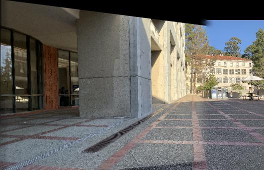
Final Panoramas
My final panoramas use the same stitch function as before and I use the same blending. As we can see, I get similar (perhaps better results) for the Lewis courtyard example!
What I learned
Through this part of the project, I learned all the fun tricks that are used in image stitching. I particularly enjoyed the RANSAC portion because it was a neat statistical trick that isn't based purely on pixels. I think the coolest thing I learned is how far pure feature descriptor matching can get, even without rotational invariance! I also saw that smaller pictures worked remarkably better for this. Not only were all the methods a lot faster, but perhaps because the feature descriptor covered more space, I was able to get great results! To me, this differs with the point in the paper how showing that 40x40 sized down to 8x8 works best.