Overview
In this project, I played around with different image morphing techniques involving warping
and interpolating colors to combine multiple images.
Shooting Images
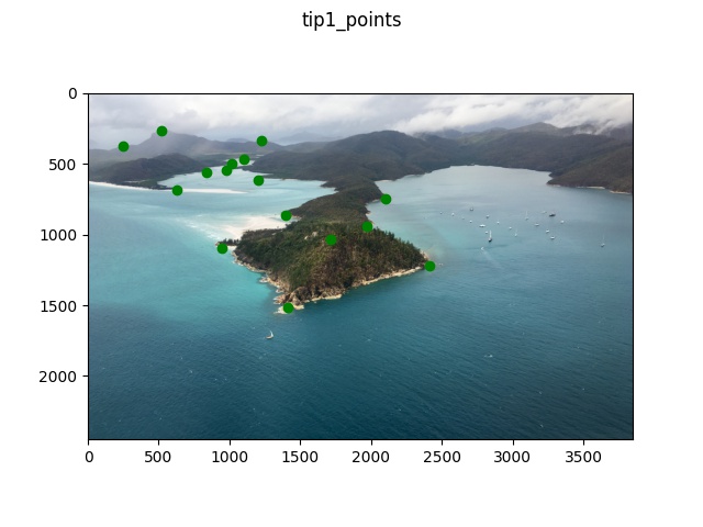
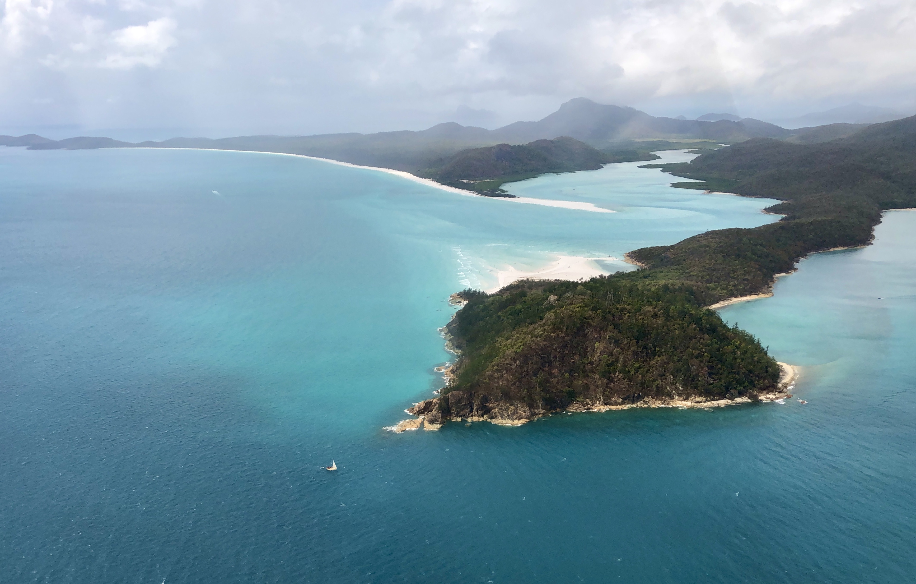
 Whitsundays 1
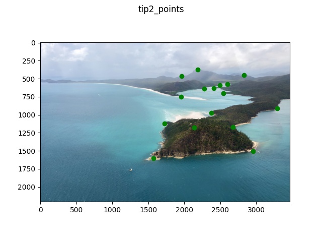
 Whitsundays 2
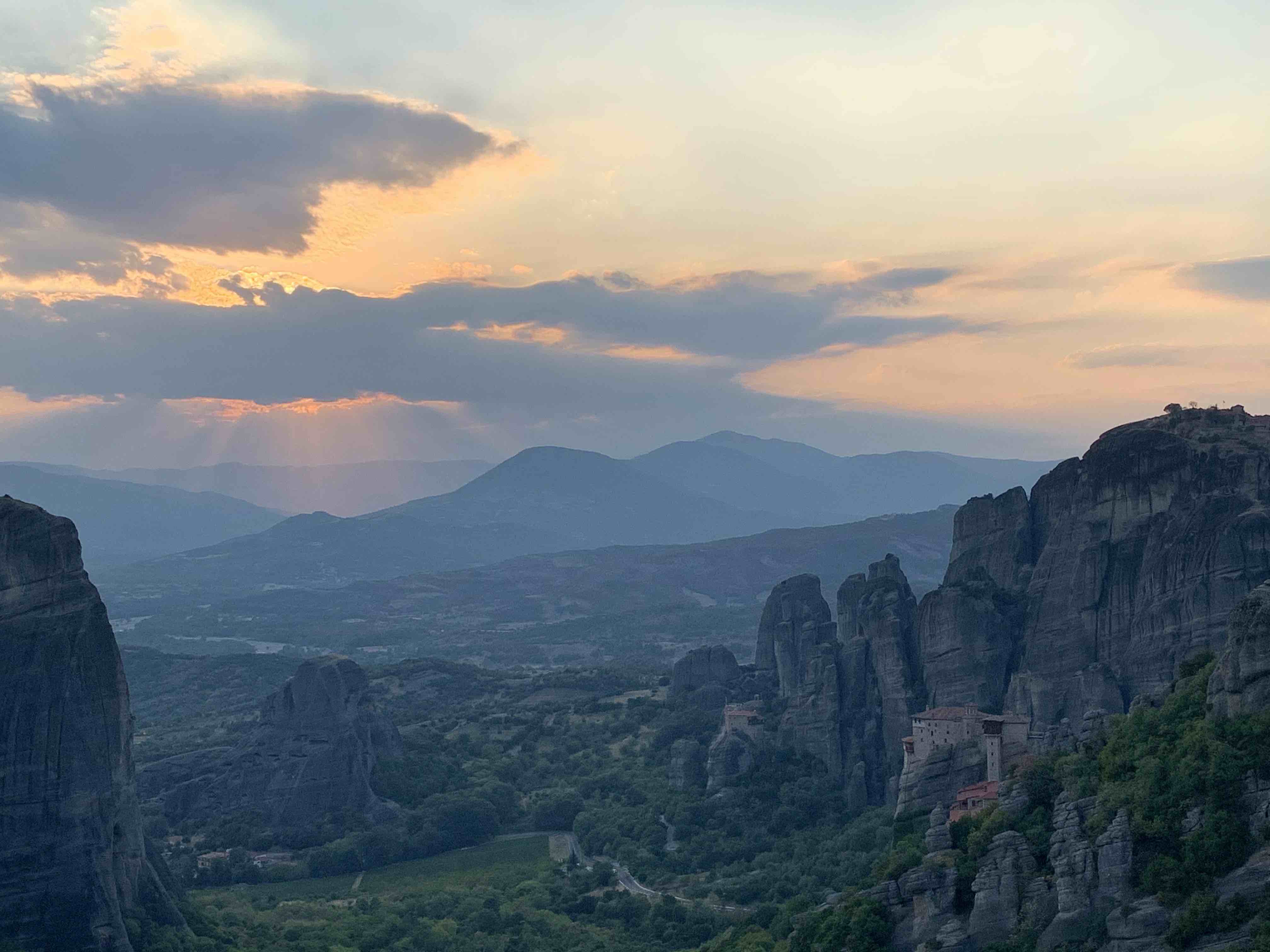 Meteora 1
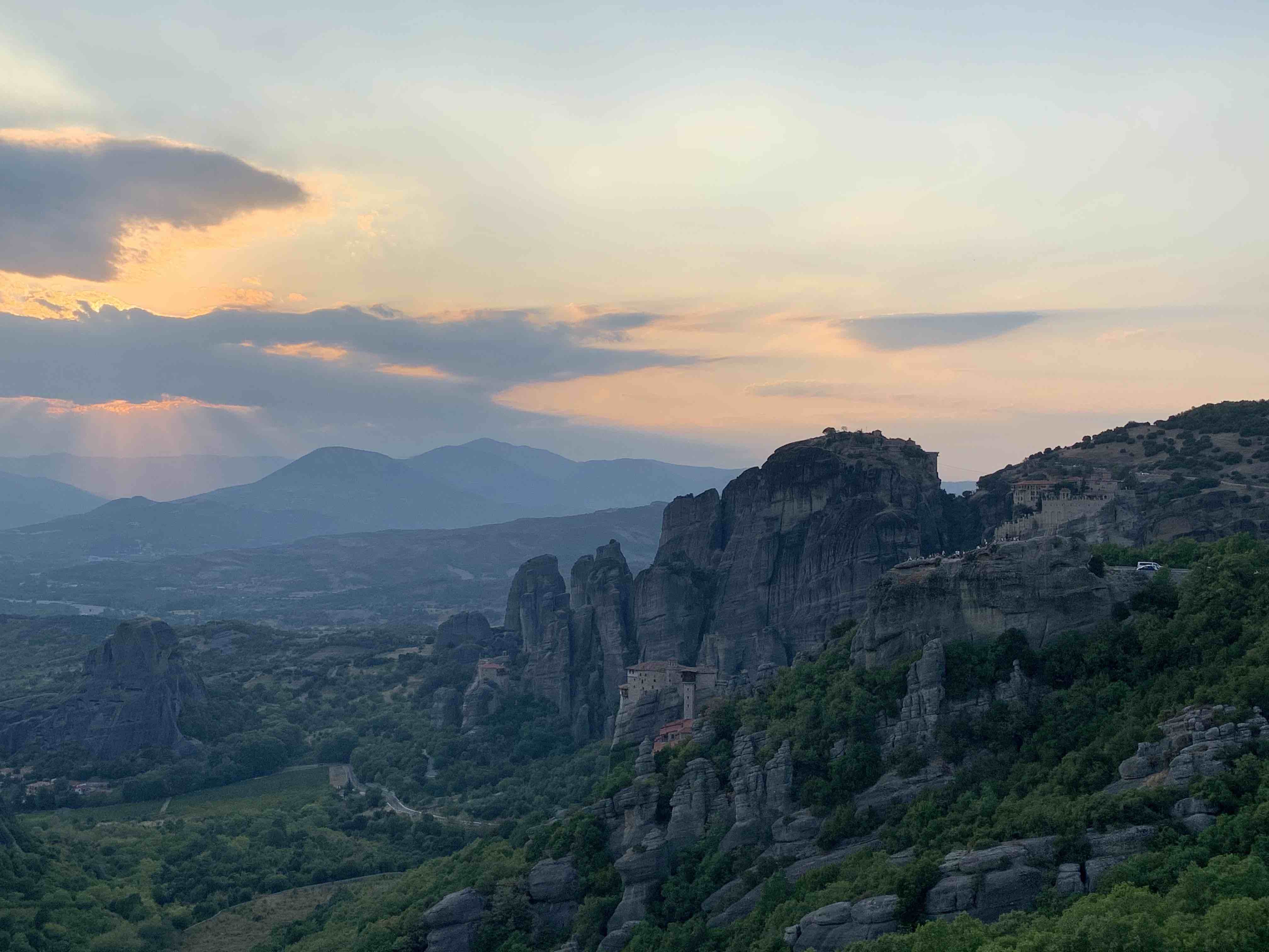 Meteora 2
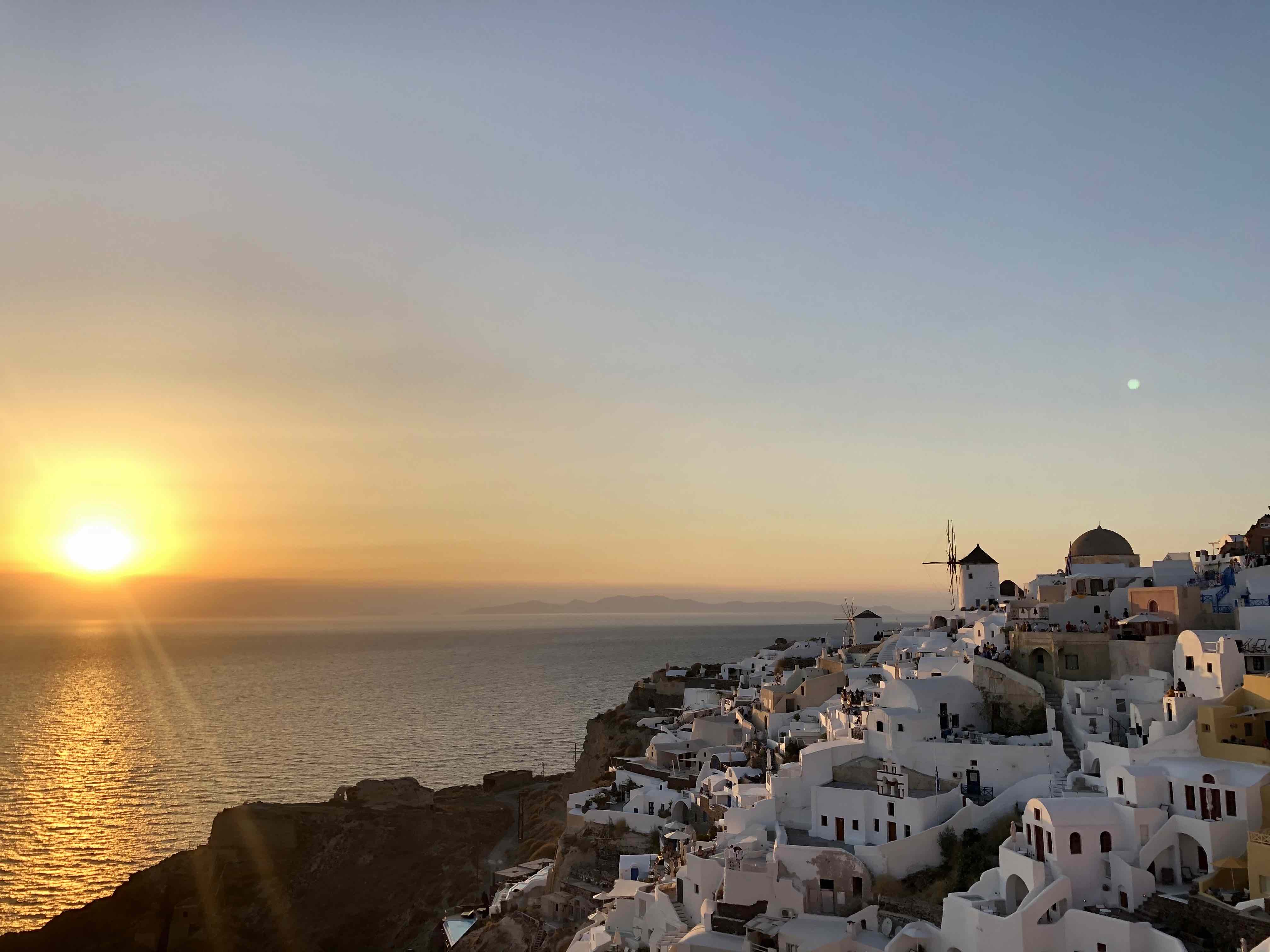 Santorini 1
 Santorini 2
 Santorini 3
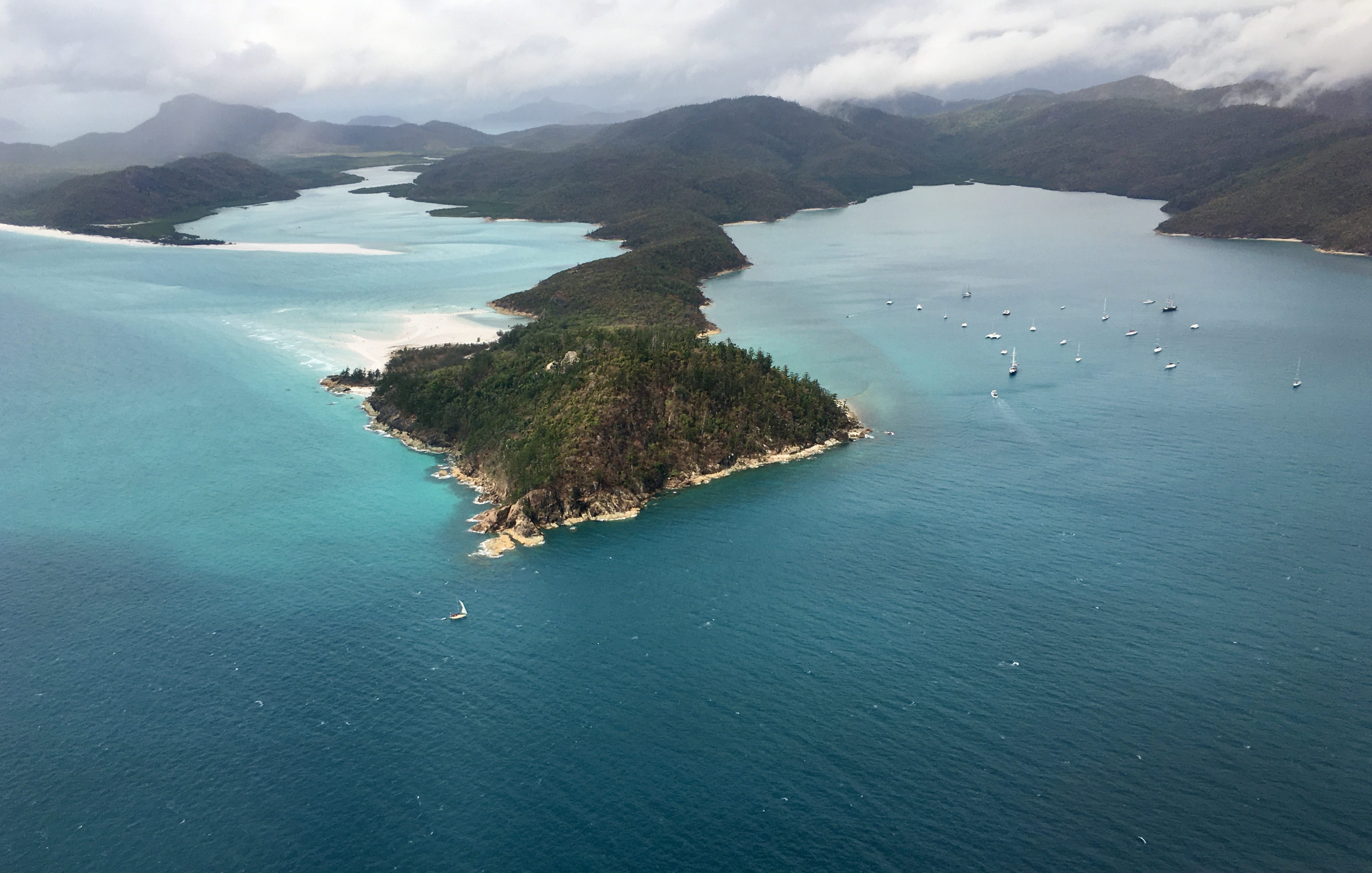
Here are the images I shot during some of my favorite vacations. Each of them shows a scenic
view from a slightly different perspective.
Recovering Homographies
Here are the point correspondences that I selected for the input images.
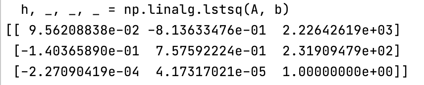
Using these points, I calculated the homography matrix. To do so, I set up a system of equations
where I created a matrix A and b and solved for the appropriate 8 degrees of freedom. The matrices I created looked
like the following where x and y are the points of image 1 and x-hat, y-hat are points in image 2:
 matrix A
 vector b
With these two matrices, I set up the system of equations Ah = b. Since I had a lot more points (> 8) than necessary, the
system of equations might not have an exact solution so I used least squares to solve for the best vector h. I then added a
final value of 1 and reshaped h to create the final appropriate homography matrix. The following image shows the resulting
H matrix which I created using the above two images and correspondence points.
Warp the Images
I decided to warp my second image onto the first image. To do so, I multiplied the coordinates of
my second image with the inverse of the homograpy matrix and then performed remapping/interpolation of the
image to project the appropriate colors onto the new basis. The result was as follows:
Original 1
Original 2
 Image 1 projected onto image 2's correspondence points
Rectify
For rectification, I chose two images I took at the Getty museum that were not completely
front-facing. The original images come at a slight tilt and I selected the edges of the potrait frame and ceiling window respectively
and projected both onto a straight rectangular region to make the image appear front-facing. The result was quite nice!
 Original image
 Rectified image
 Original image
 Rectified image
Blending into an image mosaic
Whitsundays 1
Whitsundays 2
 Whitsundays blended
Meteora 1
Meteora 2
 Meteora blended
Santorini 1
Santorini 2
Santorini 3
 Santorini 1 & 2 blended
 Santorini 2 & 3 blended
 Santorini all blended
Here are three blended mosaics that I created. In each case, I projected one of the images
onto the other image in order to have a stable point of correspondence to project upon. For the final
three-way blend, I also projected each image onto its neighbor iteratively.
What I Learned
I thought this project was super cool because it was very interesting to learn about homographies and image
projections as a method of warping. Previously, we had worked with morphing images which used smaller
projections of triangles but I thought it was very cool that I could actually use correspondence points to
warp an entire image into providing a new perspective just by matrix transformations. I also thought it was
really cool that I was able to use a lot of the knowledge that I learned in the last two projects with morphing and
transformations and apply them in a new setting where I was able to create cool blended images that stitched
together multiple perspectives.
Overview
In this project, I learned how to do automatic feature point detection using the following ensemble of
methods to identify corner features, filter out good spatially located points, and finally perform matching
and feature detection between images.
Harris Points
Image 1
Image 2
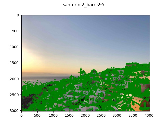 Image 1 Top 95% points
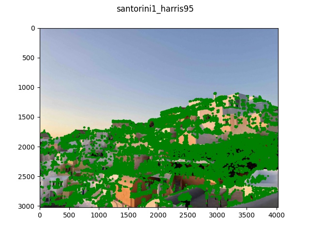 Image 2 Top 95% points
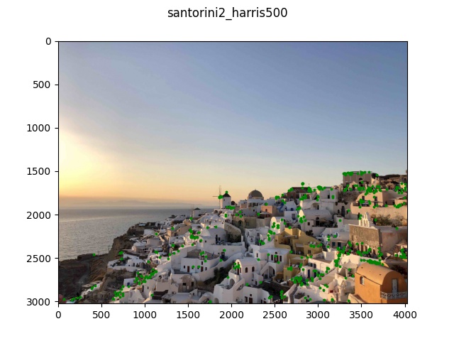 Image 1 Top 500 points
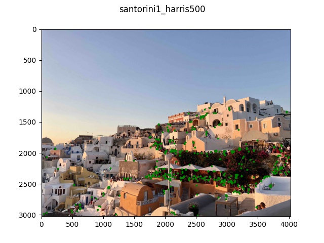 Image 2 Top 500 points
In the above images, I used the default harris function provided in the starter code. I noticed that
the provided peak_local_max function already handles finding the best point in a 3x3 region; however when
graphing all of the identified harris points, the image I took had a pretty high original resolution so the
entire picture was quite literally covered in harris points and you could barely see the image. Therefore,
for the remainder of the project, I filtered out only the top 5% of points that had the highest h-values and
only used those for future calculations. I also showed the top 500 points in h-values as a reference for the next
part where I identify the best 500 spatially located points.
Adaptive Non-Maximal Suppression
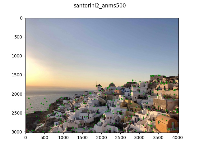 Image 1 ANMS 500 points
 Image 2 ANMS 500 points
For each image, I implemented ANMS which took in the top 5% of points (from the previous part) and
calculated the minimum distance between every point and its closest neighbor that was within 0.8 * h_value (of neighbor).
This would mean that the largest h-value point had min distance infinity and every resulting point in sorted order
would calculate its distance with preceding points in the sorted list (as long as those points were at least h_value < 0.8 * h_neighbor).
Then, among these distances for each point, I selected the top 500 points with the maximum distance to ensure that the
most spatially distanced points with highest h-values were selected.
Feature Descriptors
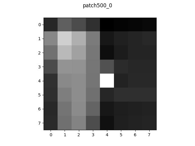 Patch 1
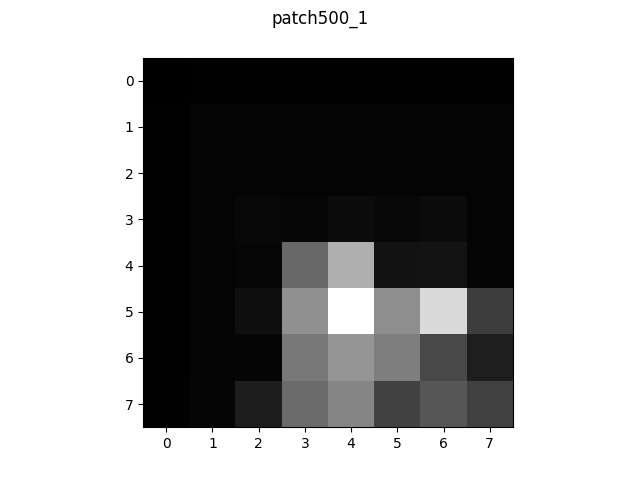 Patch 2
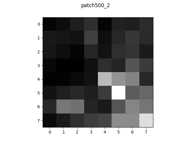 Patch 3
 Patch 4
Here are some example patches I created for each point selected from ANMS. The patches were the result of
extracting a 40x40 region around each point, performing a gaussian filter convolution to blur the image, and
then downsampling by every 5 pixel to produce the 8x8 patch.
Matching
 Image 1 matched points
 Image 2 matched points
Looking at each point's patch, I calculated the squared distance between each patch and every other patch
in the other image in order to perform point matching. From these distances, I found the nearest and second-nearest
patches to each other and kept only the points whose distance ratio between nearest and 2nd-nearest neighbors were
small enough below a threshold. This ensured that only points of relatively strong confidence were kept. We can see from
the image that for the most part, a lot of the kept images are really similar between the two images.
RANSAC
 Image 1 matched points
 Image 2 matched points
The last part of the feature detection process is RANSAC. I used the 4-point algorithm discussed in class
where I continuously sampled 4 random points and calculated the distance between all points using the homography
matrix derived from the four chosen points. I kept doing this until there were 10 consecutive iterations where the
number of inliers (points that were considered "matching" since their distance was below my threshold) did not increase, which
suggested to me that after 10 random tries, we could not get any better. The results are shown above.
Feature Detection Mosaic results
Hand-picked (part a)
 Auto-detected (part b)
Hand-picked (part a)
 Auto-detected (part b)
Hand-picked (part a)
 Auto-detected (part b)
Here are the best results I achieved for creating mosaics using feature detection. On the left column, I am
showing the results from part a where I handpicked the points. On the right column are the same exact homography
transformation code performed on the automatically detected points using harris, ANMS, matching, and RANSAC. The
auto-detection seemed to perform slightly worse than my hand-seleced features because even though the algorithm was
able to identify some good matching points, the number of points at the end was a lot lower than the amount of points
I used when hand-picking so the resulting homographies were a little less aligned.
What I Learned
In this project, I learned a lot about feature detection and methods to both extract important features and also
perform robust matching. The most imteresting thing I learned was probably how to create feature descriptors and perform
matching by doing the nearest neighbor trick using Lowe's ratio thresholding. I thought that was a really neat way
to identify not just the most similar points for matching but also the best point since we don't solely measure a match with
the nearest neighbor but with the point that is most similar to the nearest neighbor and most different from the second-nearest.