Image credit to this website
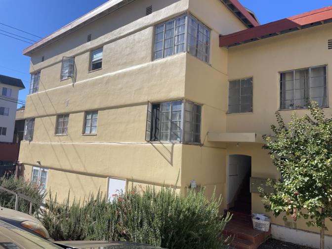
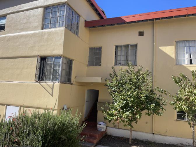
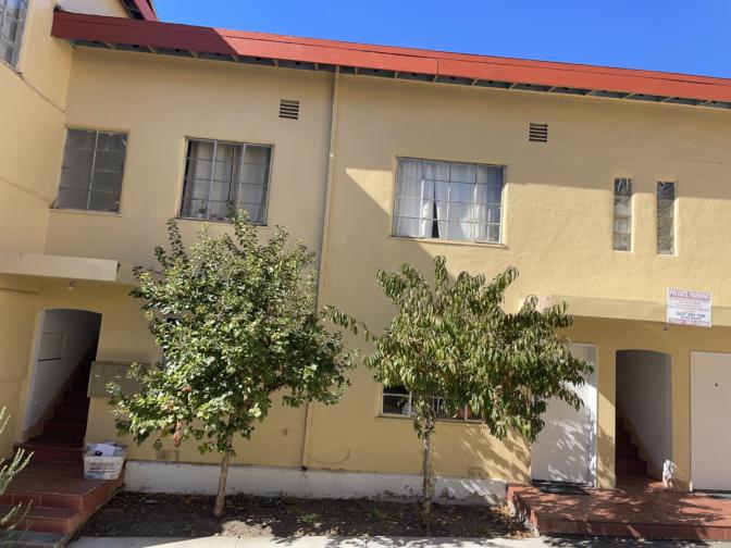
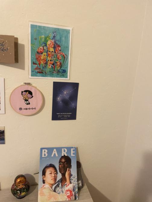
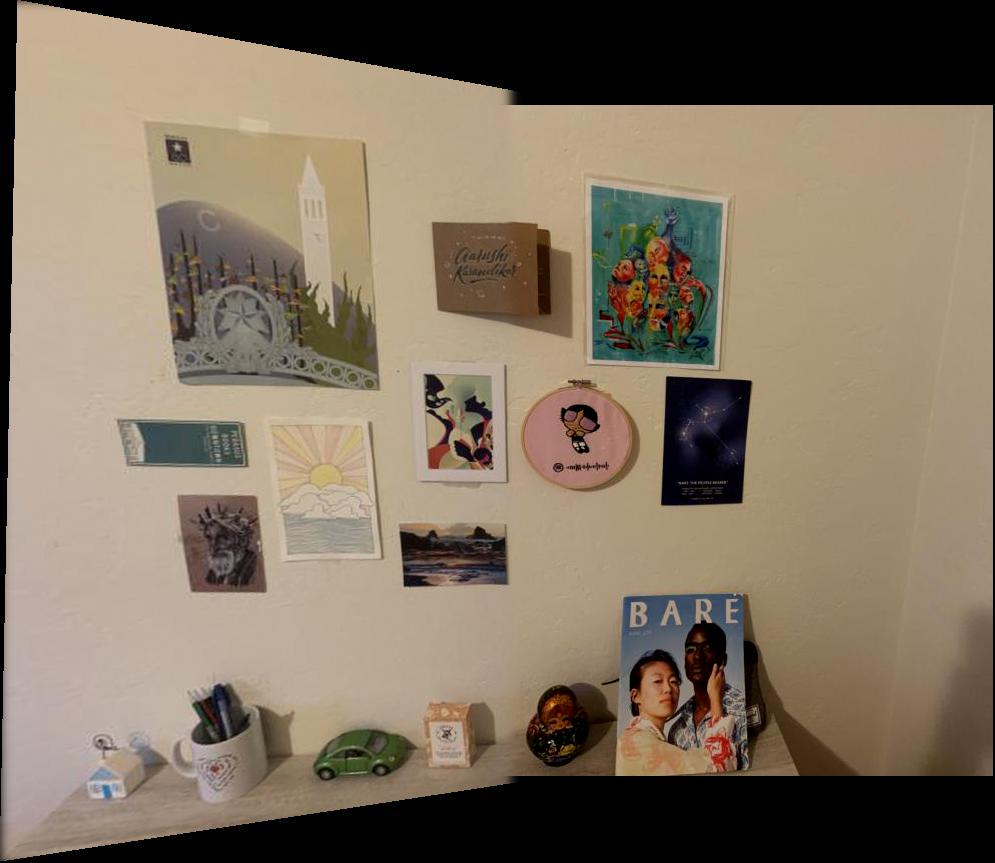
I took all of my photos on my iPhone and ensured that the aperture and exposure settings remained the same across any series of photos by taking a "burst".
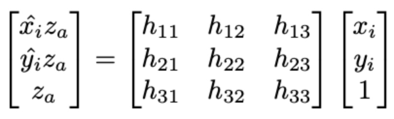
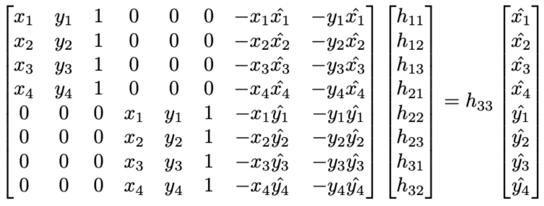
In order to recover the homography, I unraveled the homography change of basis (see above) into a system of linear equations (see below). I knew that I would want to use more than 4 correspondences for most of my images, so I wrote my code to construct this linear system to generalize to any number of correspondence points, and then solved the system with least squares.
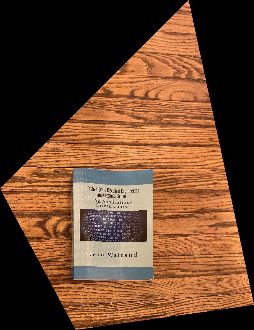
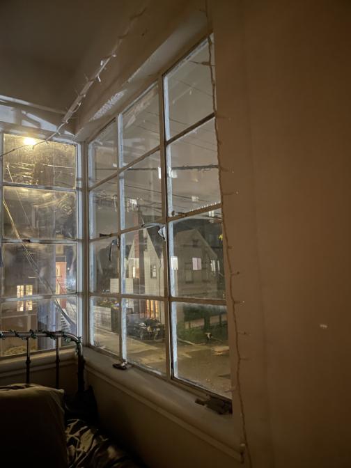
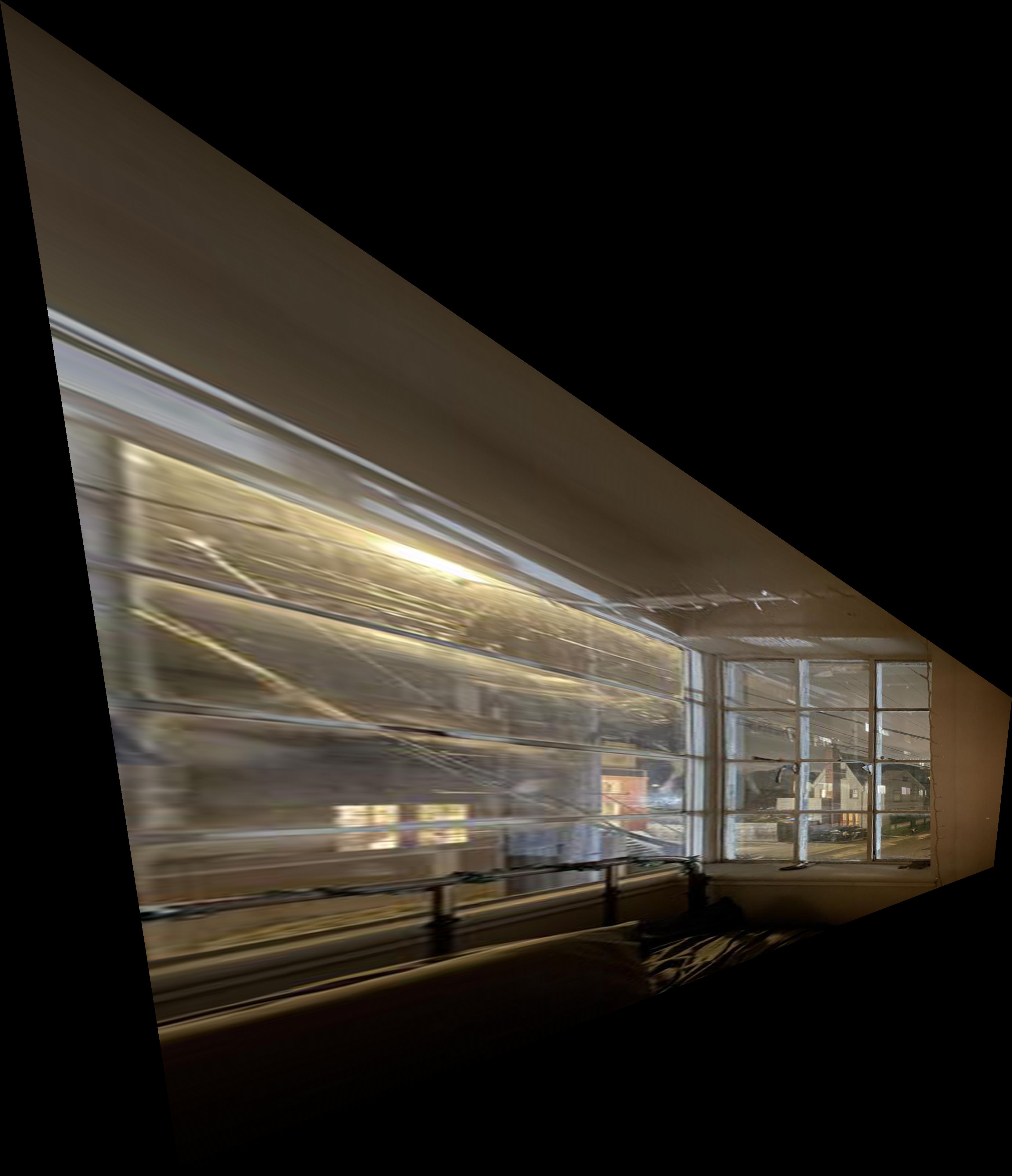
To rectify an image, I first recovered the desired homography transformation and then performed inverse warping with linear interpolation to obtain the pixel values in the final warped image. This entailed first transforming the corners of the original image into the target space by doing a forward warp, in order to determine the dimensions of the final warped image. Then, I created a blank image with those dimensions and performed an inverse warp on it with a small translation, in order to obtain the coordinates to interpolate within the original image. I then filled the blank image with the corresponding interpolated points.
I was quite satisfied with the results in this section; my homography estimation and inverse warping methods were clearly working. It was cool to see how this worked in the extreme rectification case of the window (2nd example).

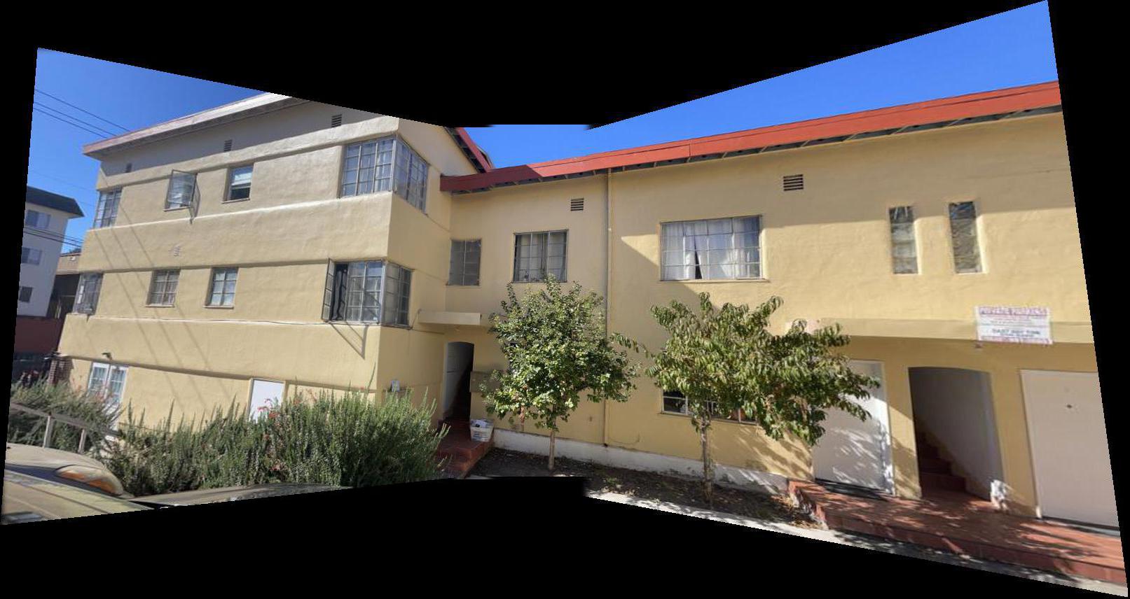
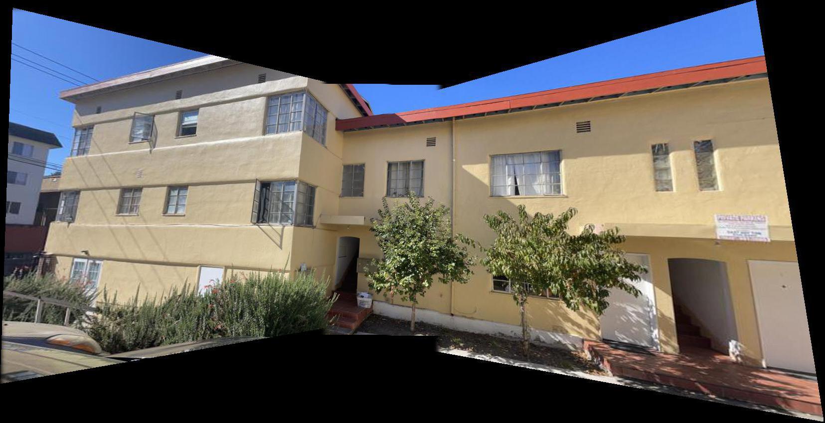
I constructed my mosaics by warping each image to another image in the mosaic. Then, I aligned each of these pairs through a simple x, y translation and finally, performed alpha blending. In the case of more than two images in a mosaic, I continue to align and alpha blend these pairs of images until one final mosaic is obtained. My code is generalized to support the alignment of any number of image pairs. My first mosaic is an example that uses three images. I was really happy with seeing all of my work come together in this result! I also love the red, yellow, and blue colors in the photo.
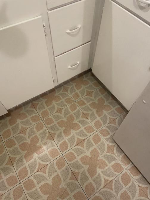
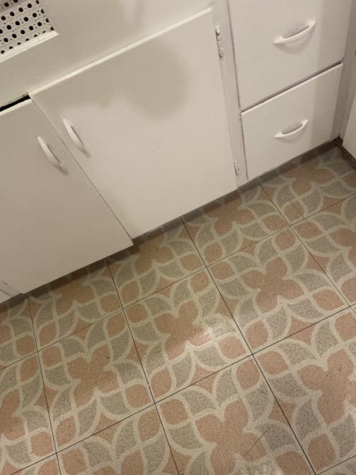
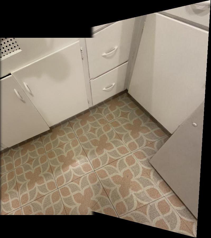
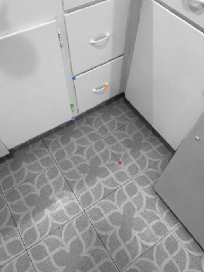
I was very happy with how flawlessly this linoleum result came out.

The most interesting thing I learned through this part of the project is how difficult it is to take photos for a successful homography estimation and application. I went through many sets of photos, but eventually found that consistent lighting and good reference points are very important features for the photos to have.
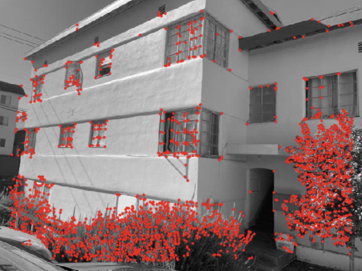
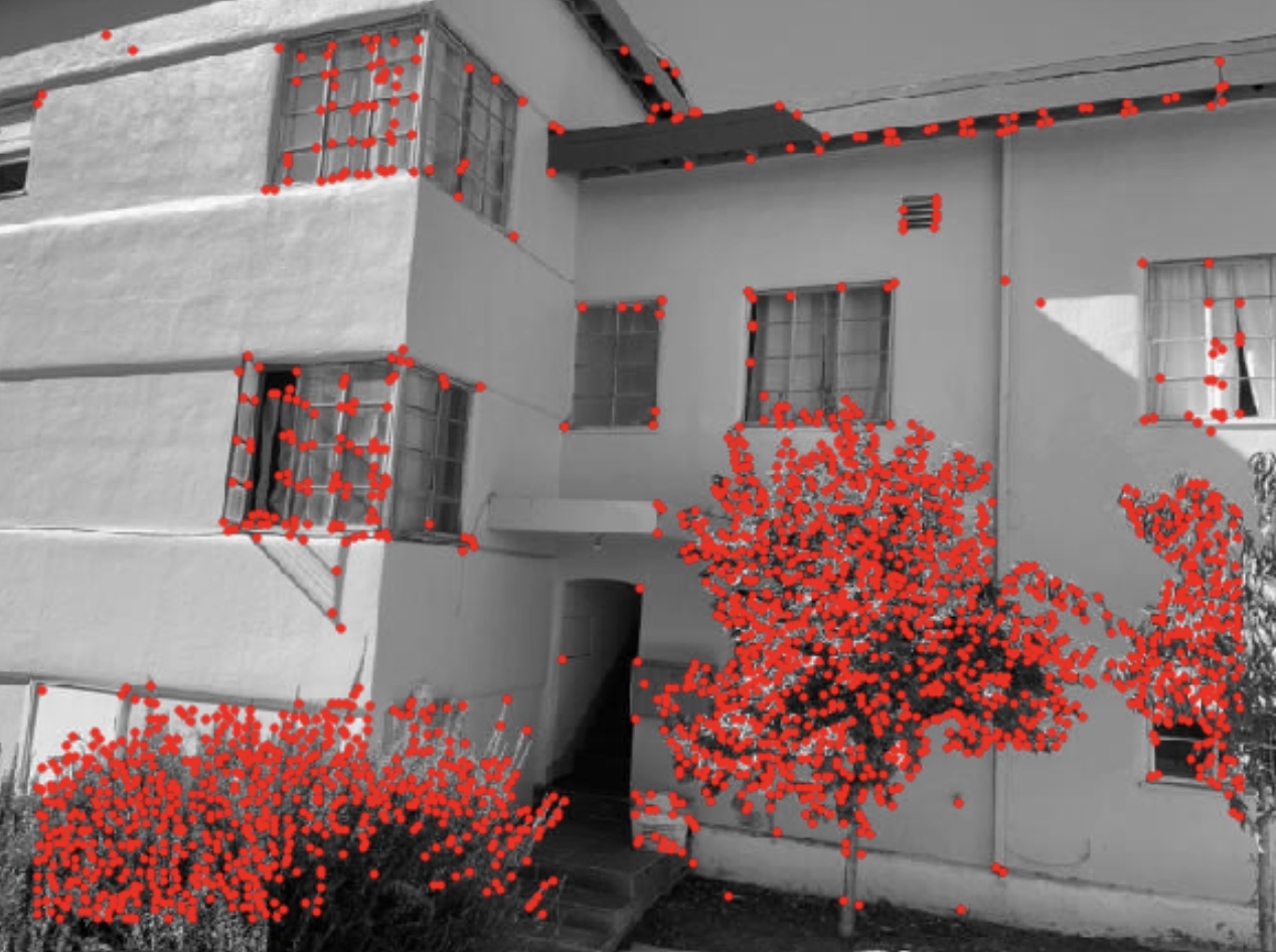
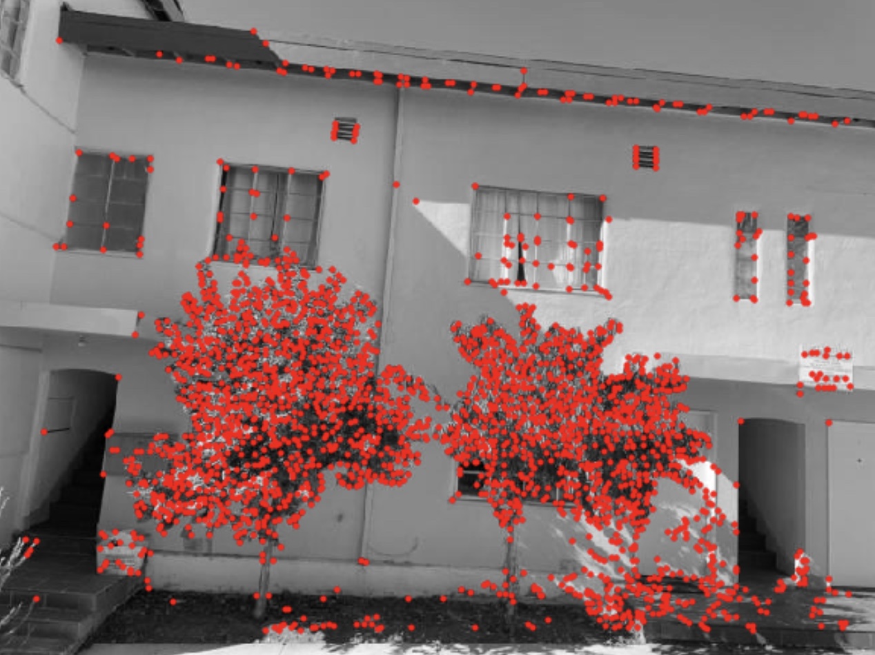
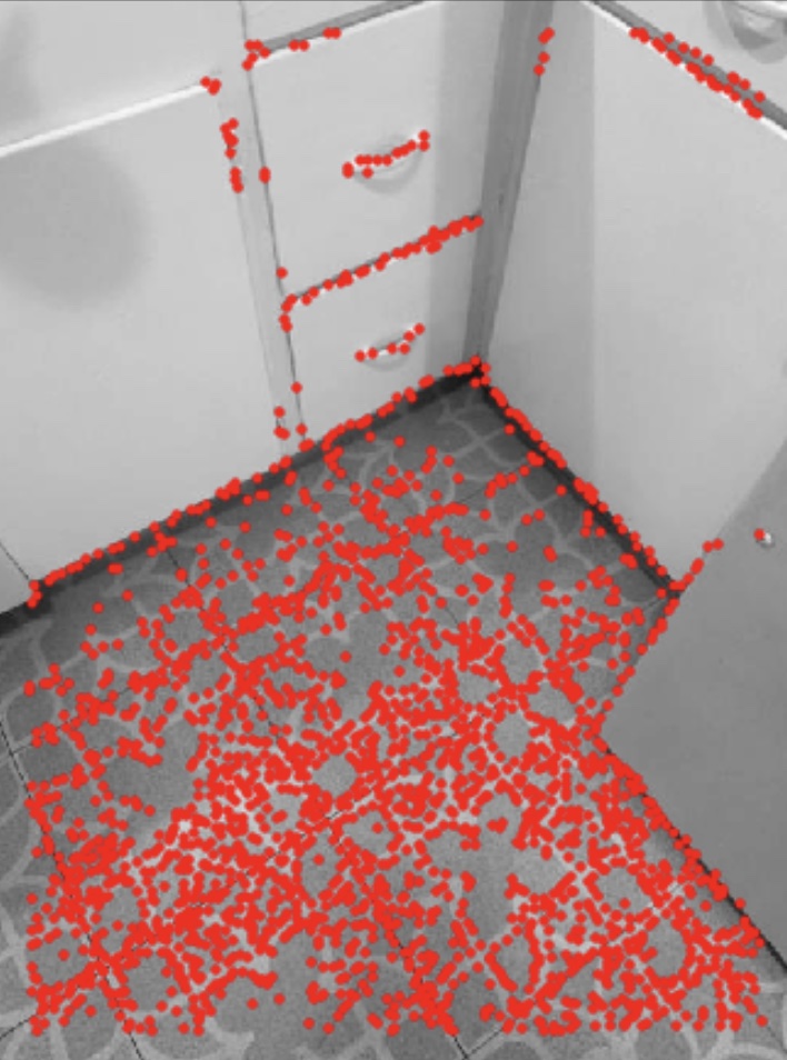
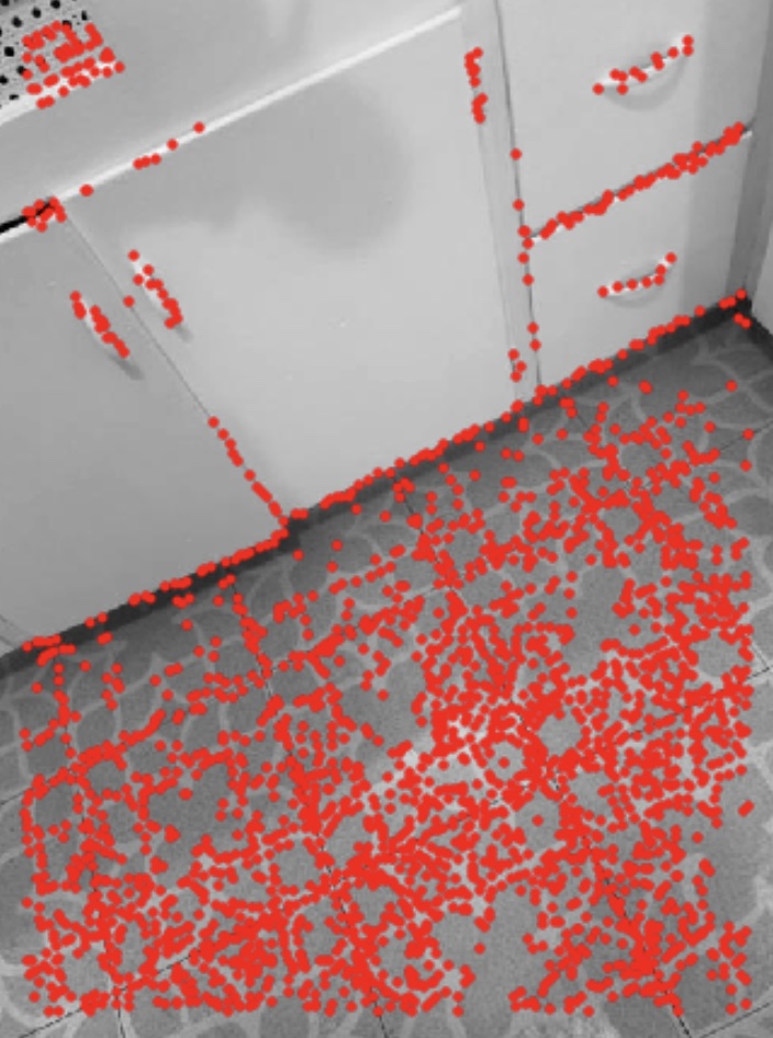
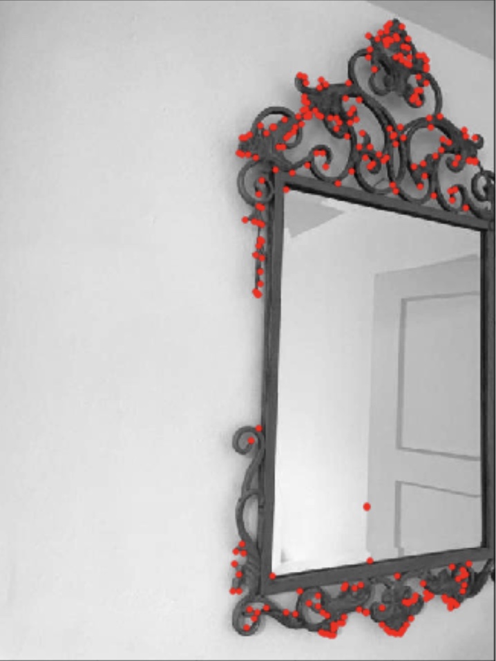
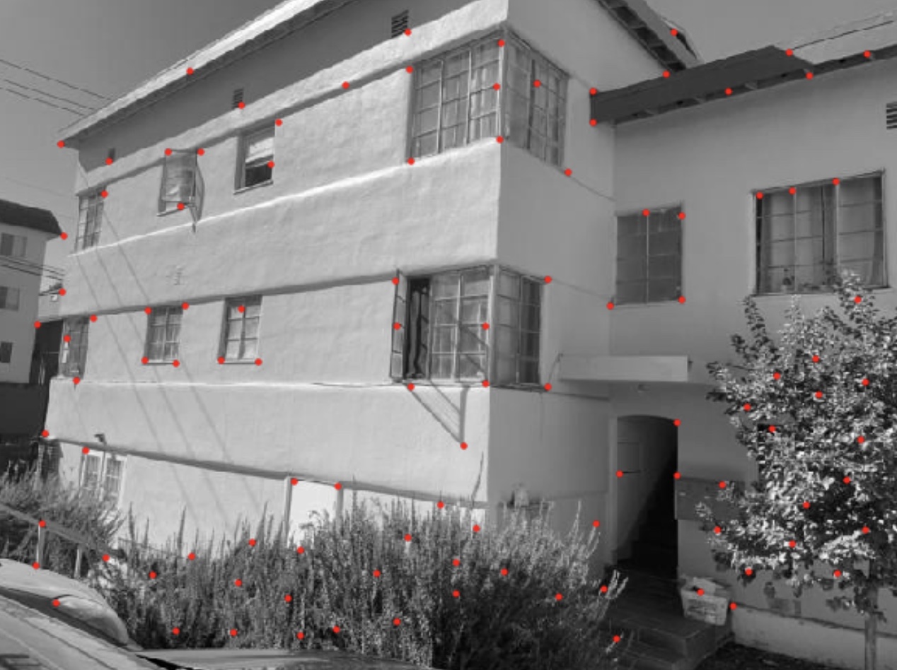
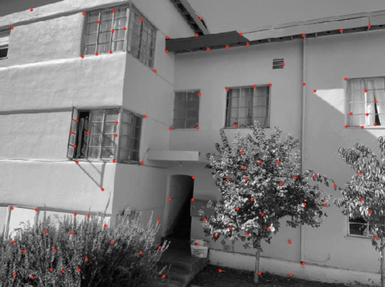
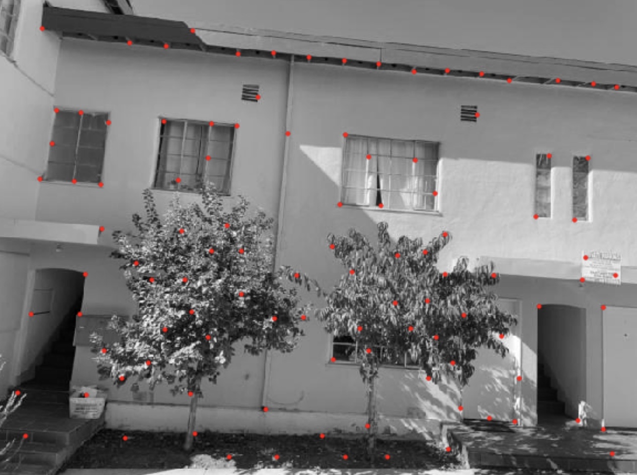
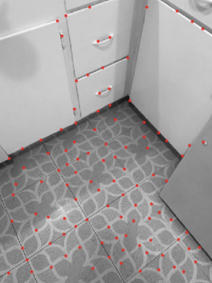
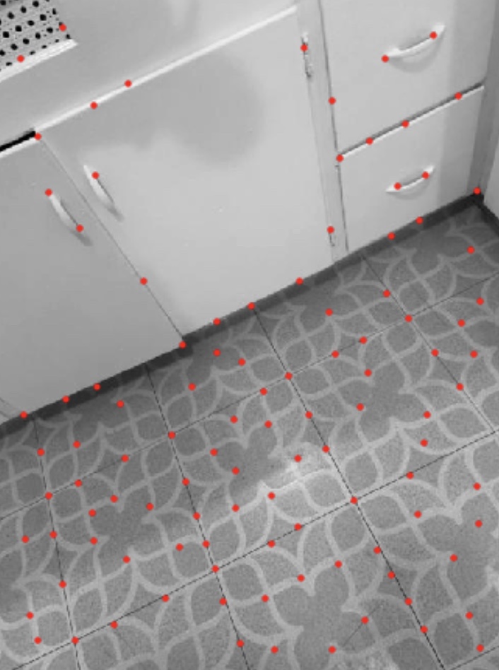
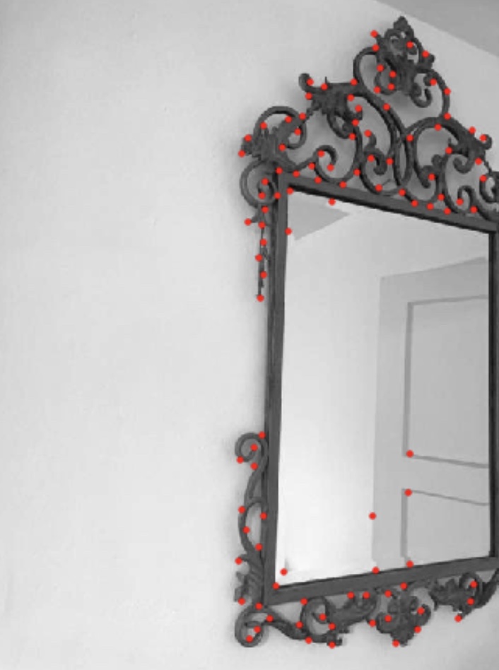
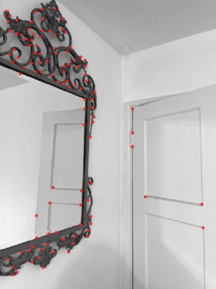
I used the Harris Interest Point Detector on a single scale and pixel-level accuracy. For this section, I used the sample code provided in the project spec. After obtaining the Harris interest points, I only kept those with a score above a certain threshold (tuned per image). I chose the threshold such that there was still a relatively even distribution of points over the entire image for my use case. I implemented this thresholding in the first place to increase the speed of the subsequent step of adaptive non-max suppression by removing points that were less likely to be chosen. The Harris interest points I kept for each set of images are shown below.

After obtaining the Harris interest points, I selected a subset of these points using the adaptive non-max suppression algorithm from Brown et al.. I implemented this algorithm by calculating the list of points ordered (decreasing) by their distance to the closest point with higher Harris score. The distance associated with the point with the highest Harris score is set to infinite. I was then able to select the number of points, m, I wanted to keep by taking the first m points of this list. The points selected by my adaptive non-max suppression implementation are shown below.
For each chosen Harris interest point, I created a feature descriptor by down-sampling the 40 by 40 patch of pixels sampled at the interest point to a 5 by 5 pixel patch. In order to implement this down-sampling, I first blurred the 40 by 40 patch using a Gaussian filter, and then took the pixel at every fifth coordinate in both the column and row directions.
After obtaining a feature descriptor for each Harris interest point, I matched each interest point from the first image to an interest point in the second image and only kept the pairs with a ("1-nn") / ("2-nn") ratio less than 0.4, as implemented in Brown et al..
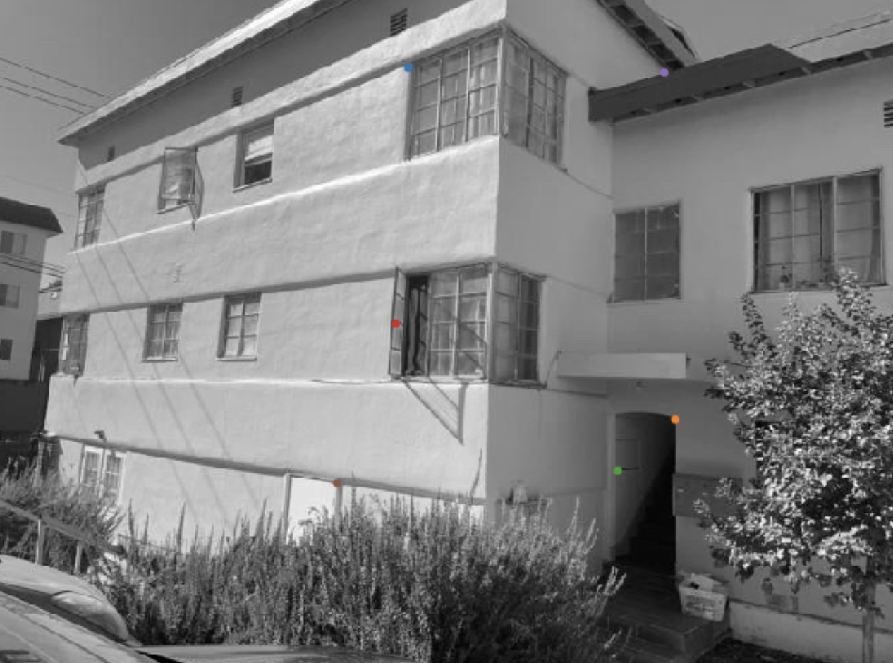
I then implemented and used RANSAC to correctly choose the point pairs for the final homography. I implemented the RANSAC algorithm as explained in class using random samples of 4 points to compute homographies and returning the inlier pairs from the homography with the highest number of inliers. I ended up with at least 5 point pairs for each pair of images. This is definitely on the lower end of the number of resulting point pairs I was expecting. There are four possible causes for this: 1) the low tolerance for error when labelling point pairs as inliers using Euclidean distance (most likely the driving cause) 2) the small portion of overlap between image pairs (definitely contributing) 3) the lack of rotation invariance in my feature descriptors 4) my thresholding of interest points by their Harris value prior to non-max suppression. However, even with this low number of resulting point pairs, I was still able to proceed to make successful mosaics.
The chosen point pairs are shown below in corresponding colors.
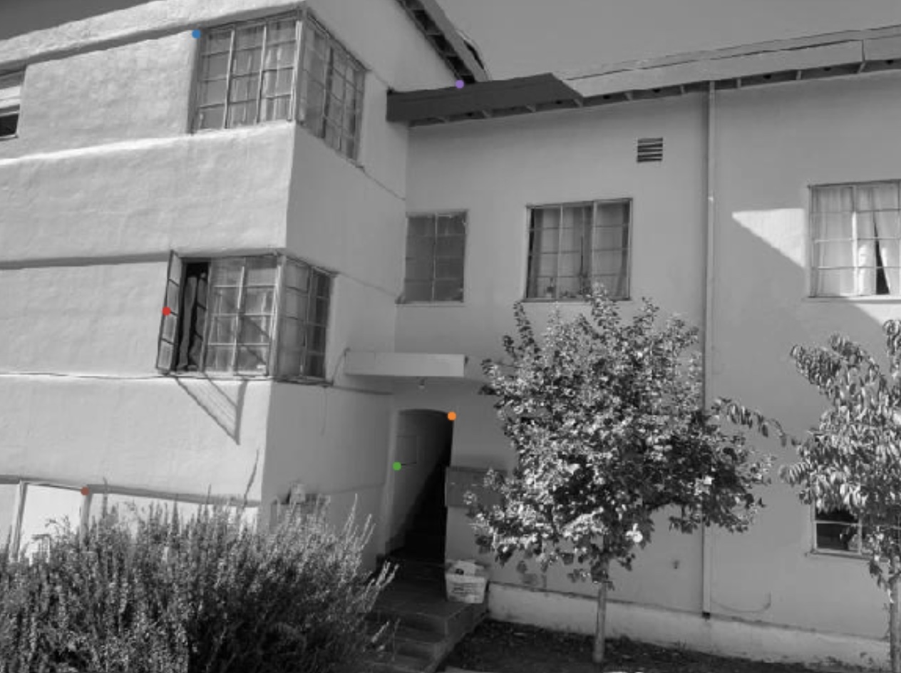
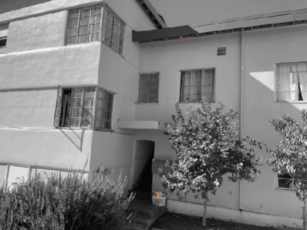
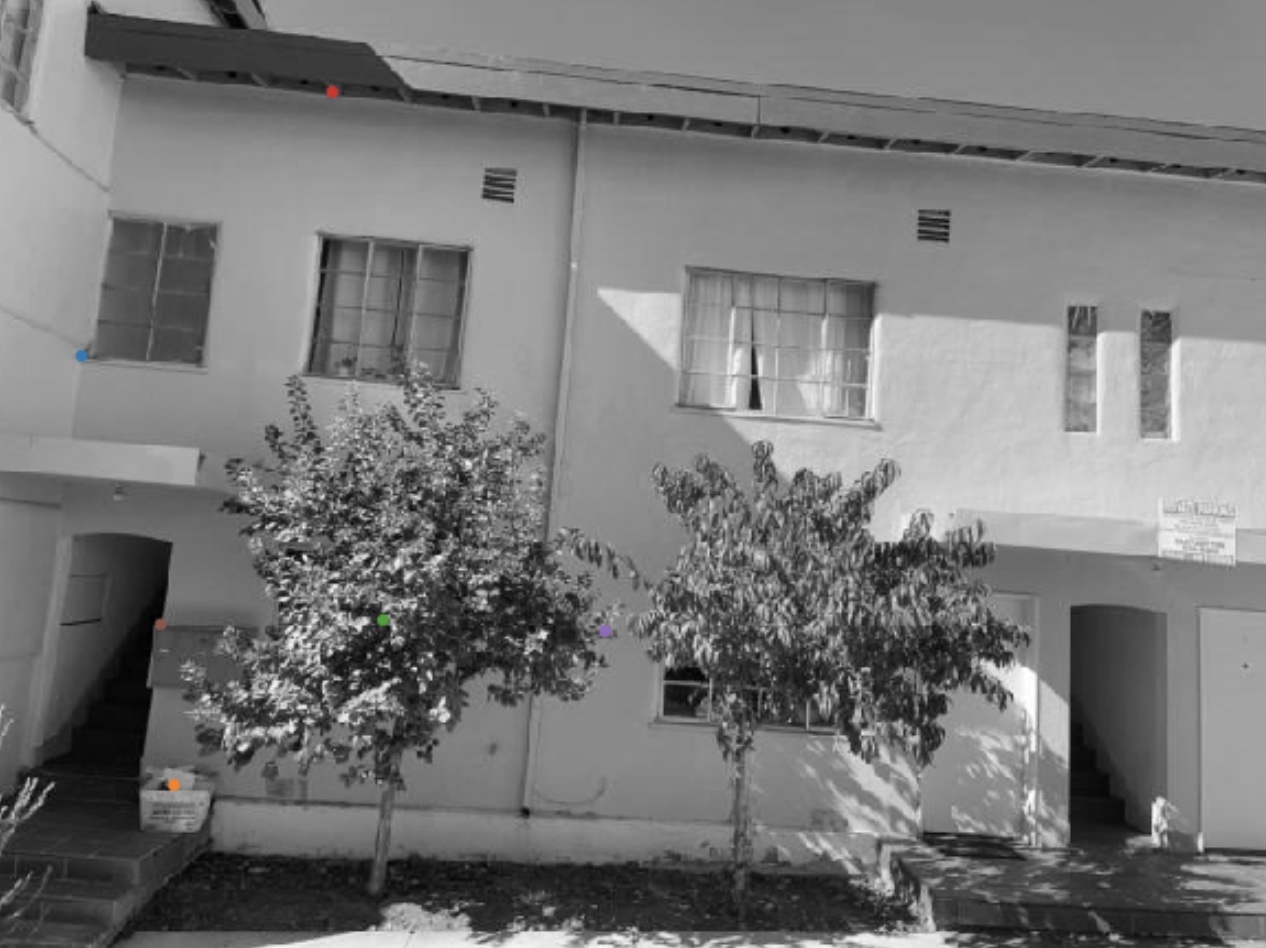
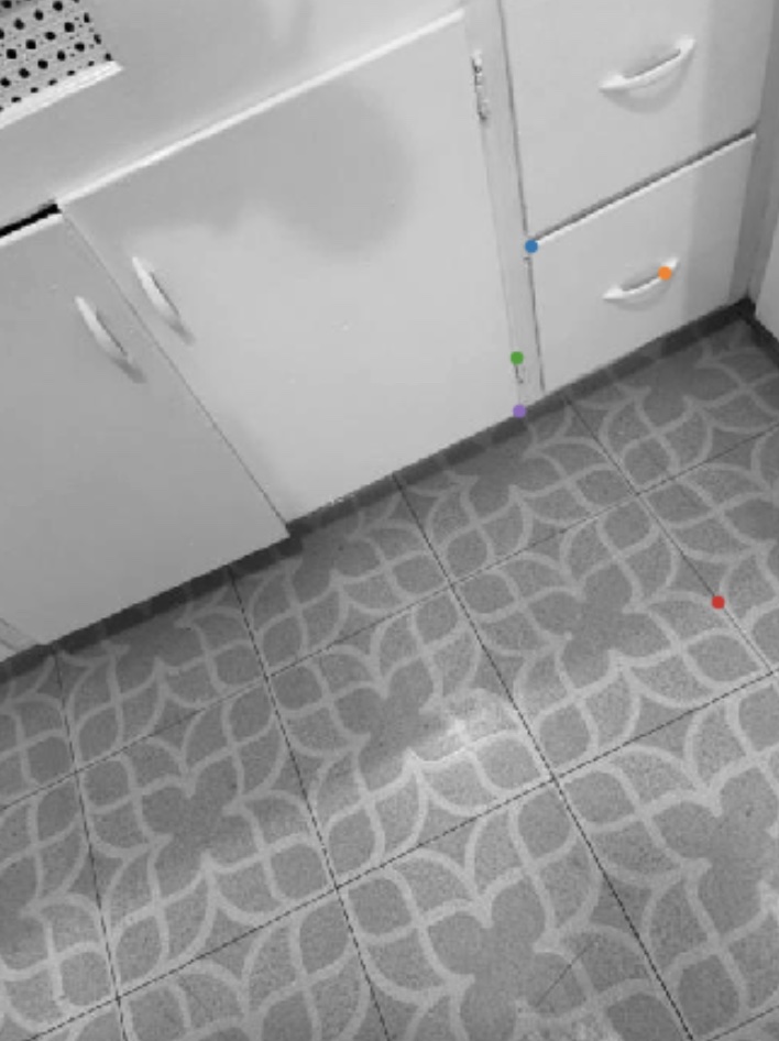
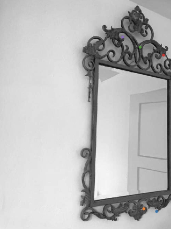
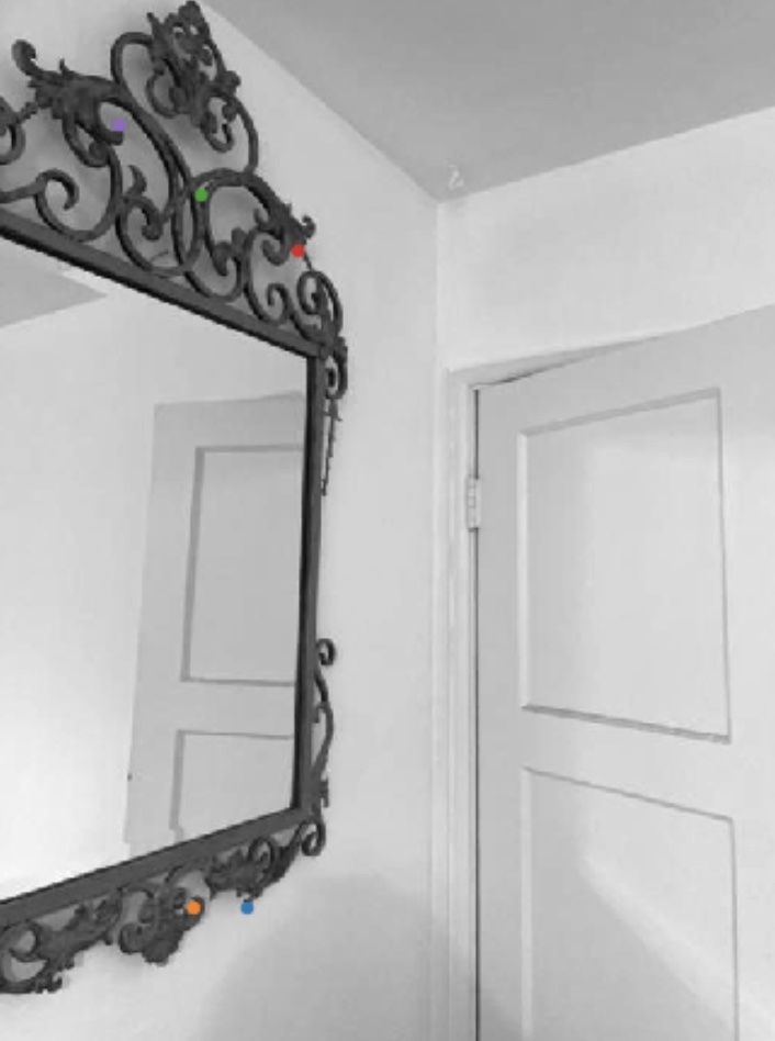
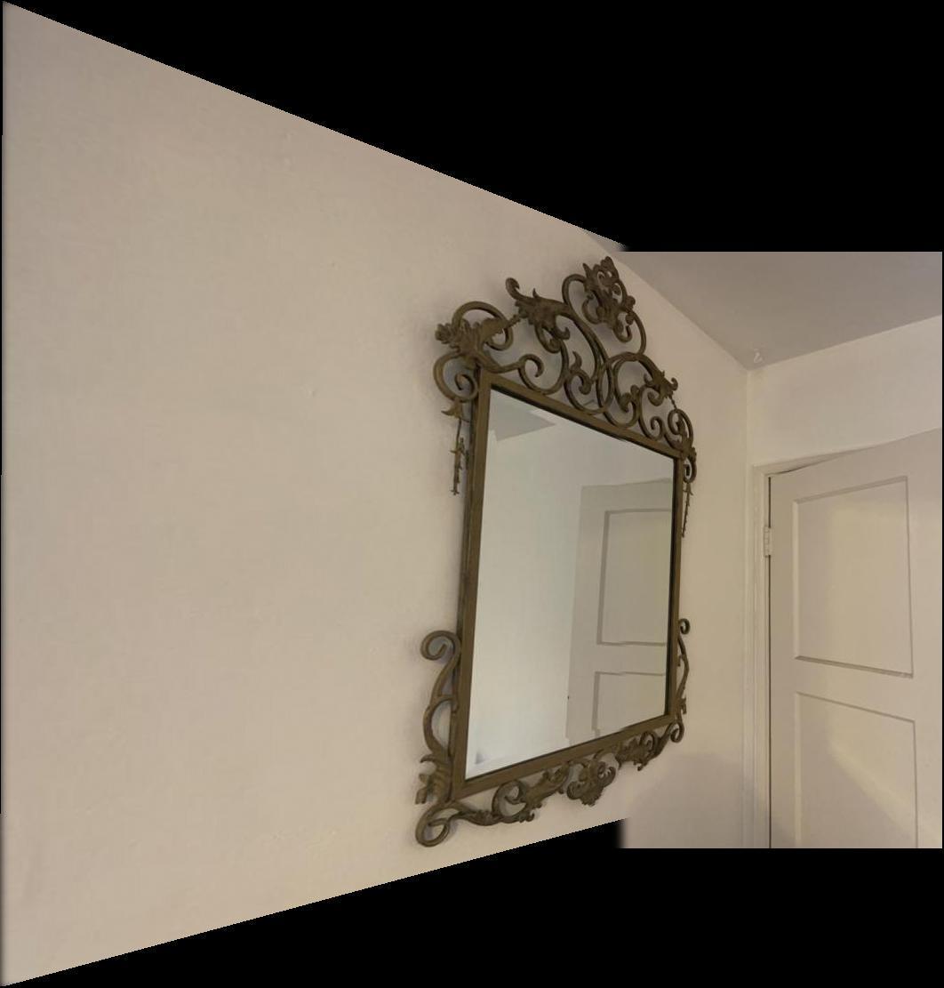
I recreated two mosaics from Part A of the project. I show these next to the mosaics created with manually-chosen correspondence points. My third mosaic is a new mosaic of a fancy mirror I inherited from the previous inhabitants of my apartment. I was pretty happy with how these all turned out for an automated process.
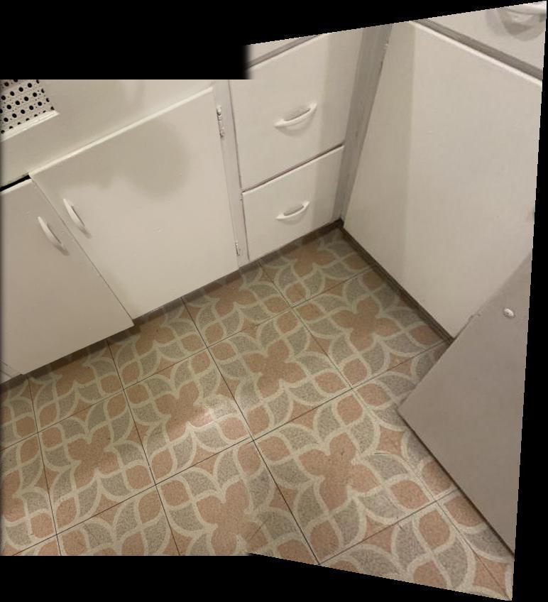
The most interesting thing I learned through this part of the project is how delightfully simple, yet effective the feature matching and RANSAC algorithms are for automatic feature matching. These are clever algorithms that are largely inspired by human intuition about how feature matching works. It was also interesting to see how the vast majority of points on the patterned tile in the linoleum photos are eliminated by the filtering on the ("1-nn") / ("2-nn") ratio. This makes sense because it is not possible for the current algorithm to distinguish between the ith and the (i+1)th tile on the floor. Additionally, the existence of the pattern means that even good point pairs in this region are ignored due to the "2-nn" error being very close to the "1-nn" error.