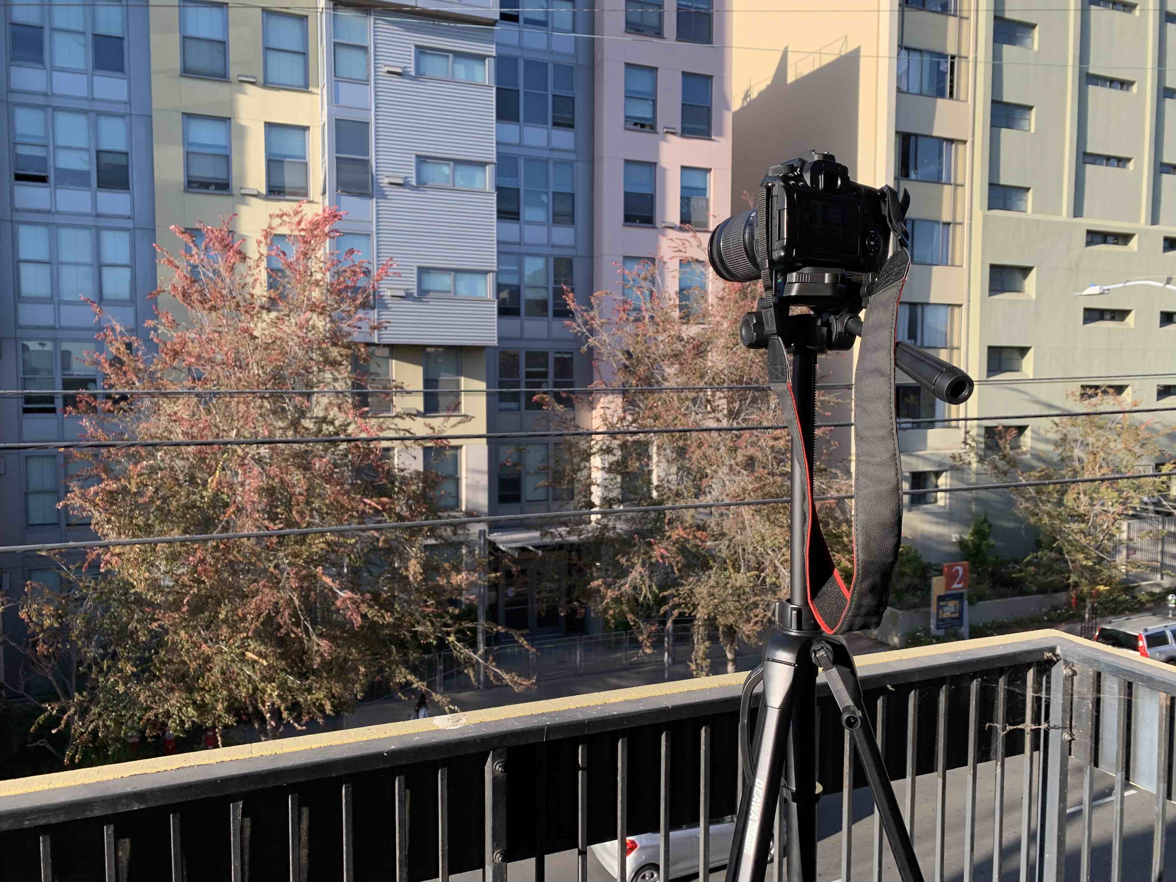
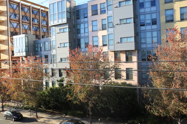
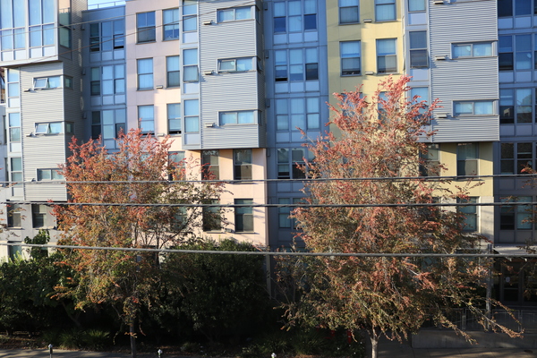
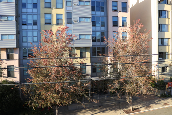
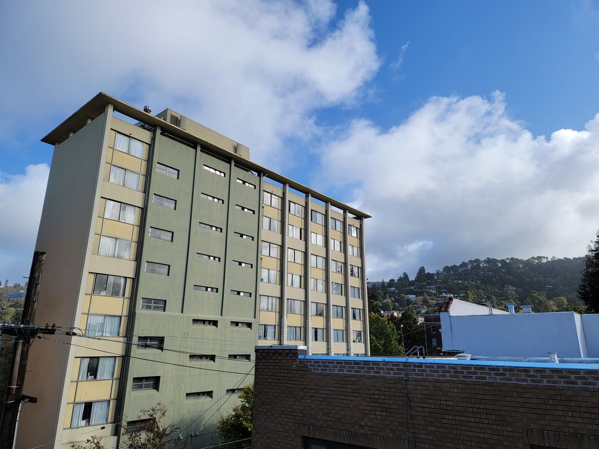
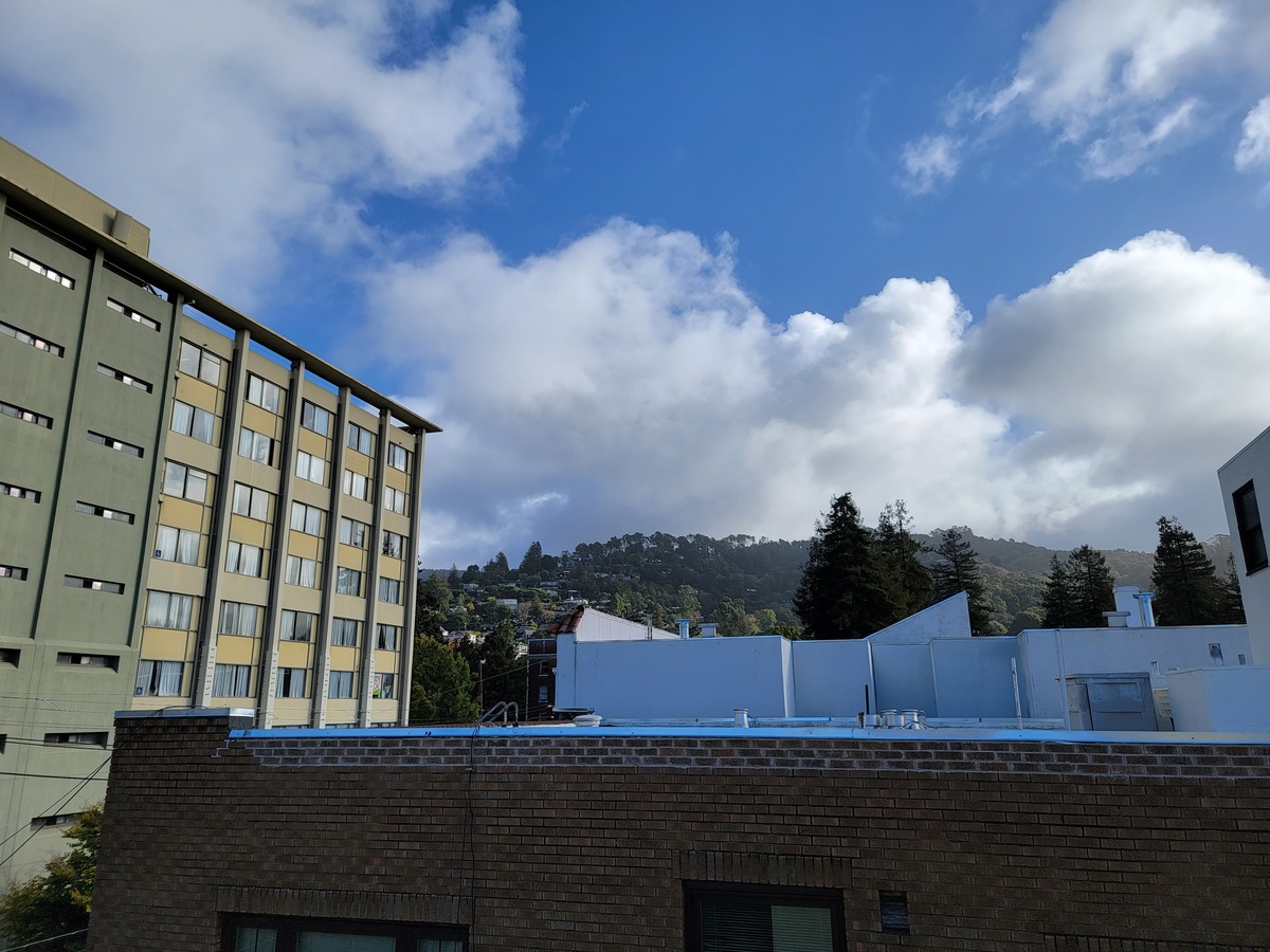
For this part of the project, I chose to use my DSLR to take the pictures (Canon EOS80D) so that I could shoot in manual mode and keep exposure, shutter speed and aperture the same (so that the photos are as consistent as possible). I put the camera on a tripod so I could turn it without translating its position and also went with a wide-angle lens as this is the typical use case for a panorama. Finally, I chose to take photos of the exterior of the Unit 2 dorm buildings in Berkeley because the windows would be easily identifiable correspondence points between the different images.
Note that all of the following images have been compressed for this website. The original images are 6000x4000 pixels each.
We know that since all the images were taken with the same center of projection and the camera was just rotated, that the transformation between each pair of images is a homography following p' = Hp, with H being a 3x3 matrix with 8 degrees of freedom (the last entry is a scaling factor = 1). If we want to recover the values of H, we can set up linear equations as follows:
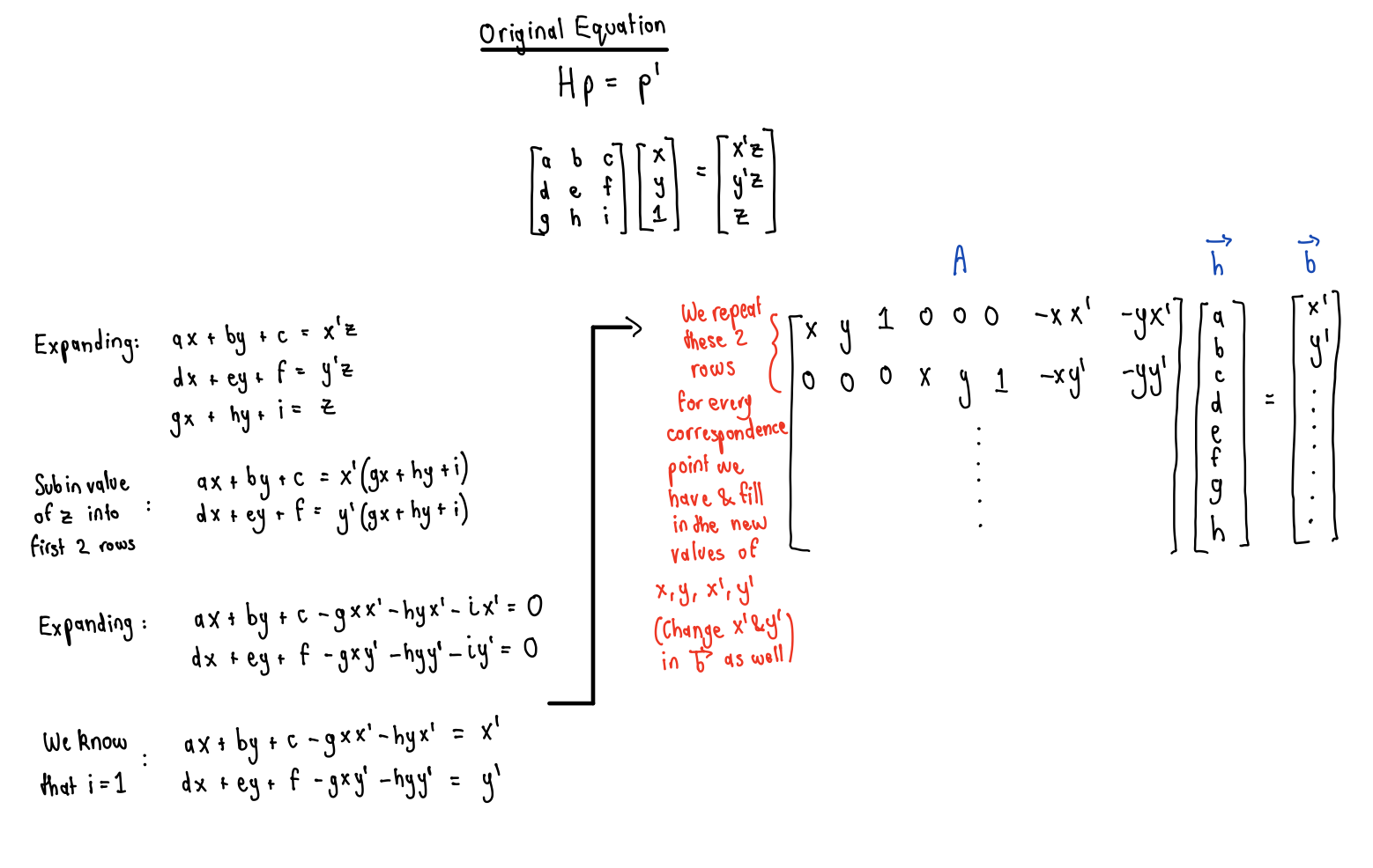
Now that we know that each (p, p') correspondence will provide 2 rows to the A matrix above, it is clear to see
that a minimum of 4 correspondences are needed. This is because this will give 8 equations to solve for 8 unknowns.
However, with only 4 (p, p') pairs, any noise in the images can lead to errors in the homography matrix. Therefore,
more correspondences were provided (E.g 8) and the A matrix and b vector were set up as above but then Least Squares
was used to find the optimal solution for the h vector.
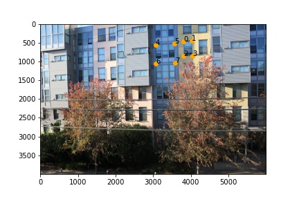
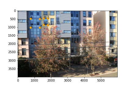
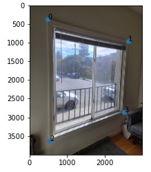
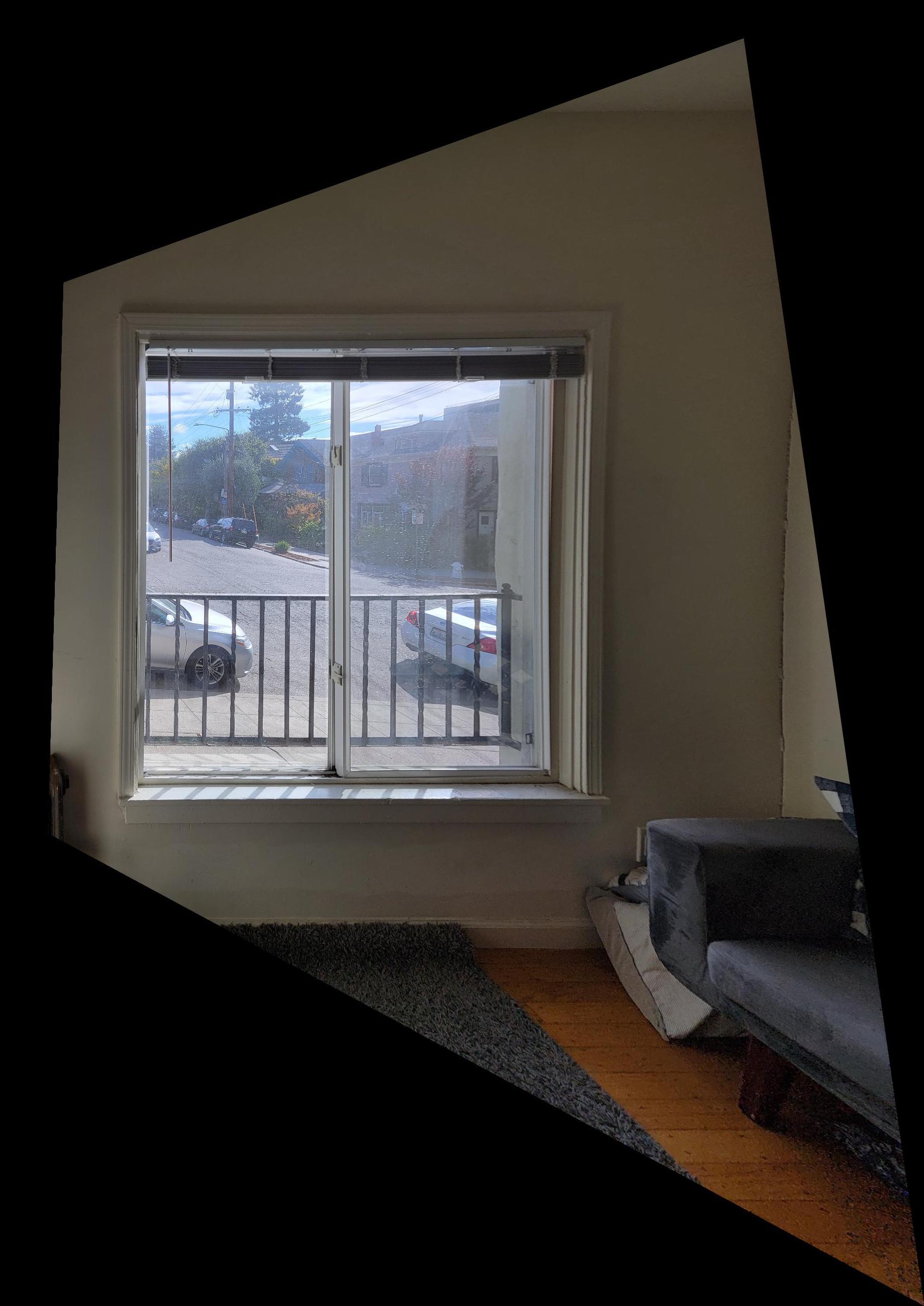
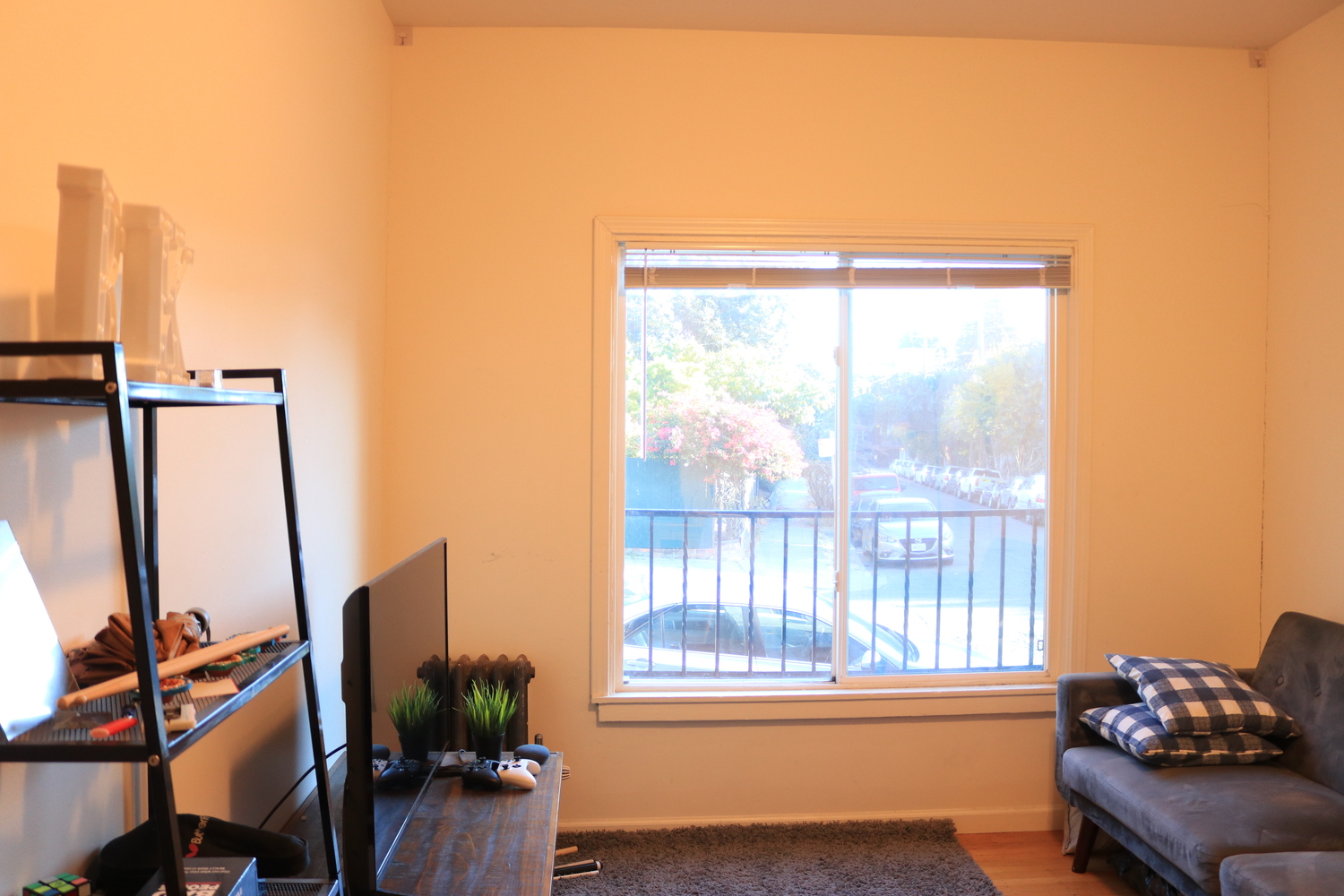
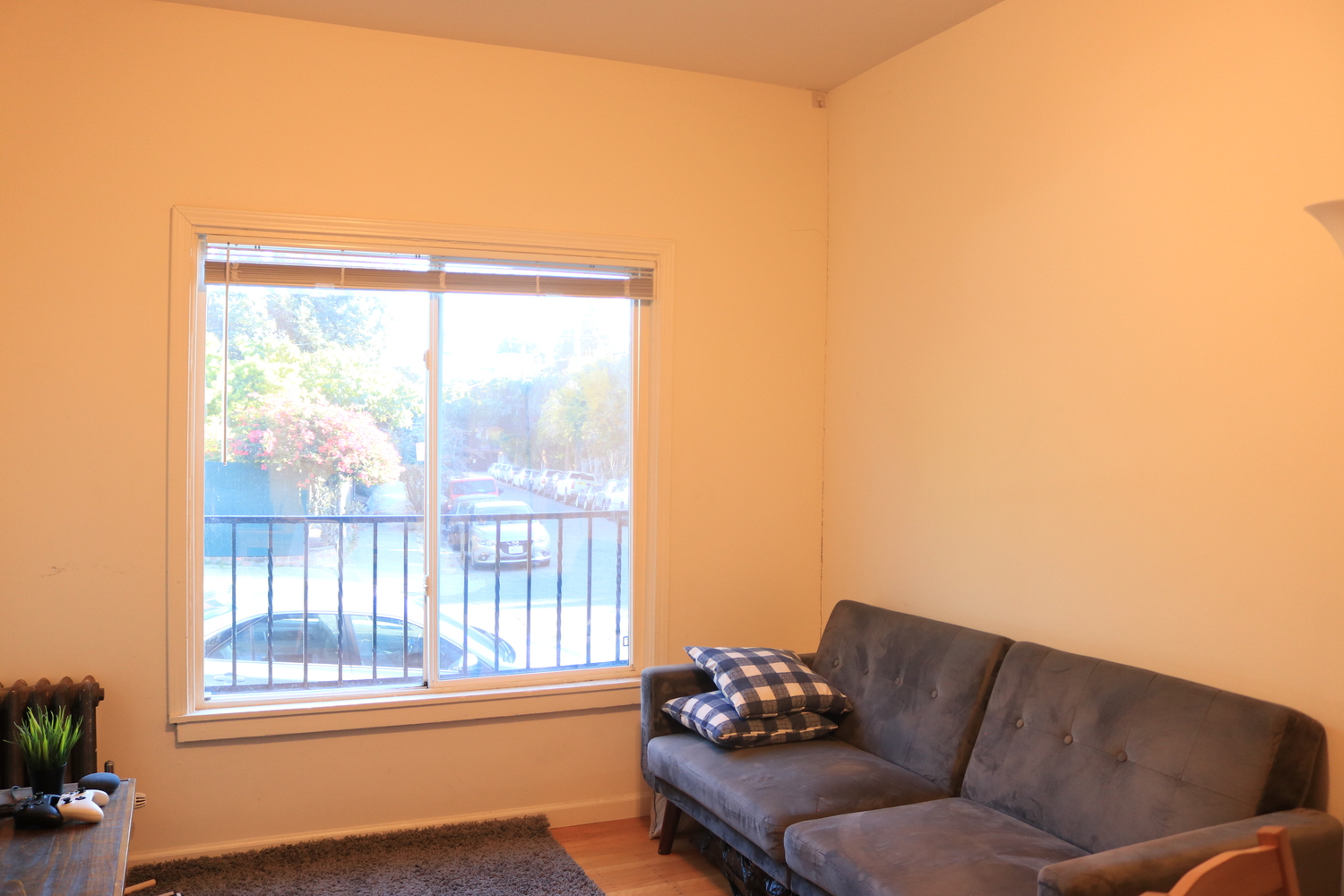
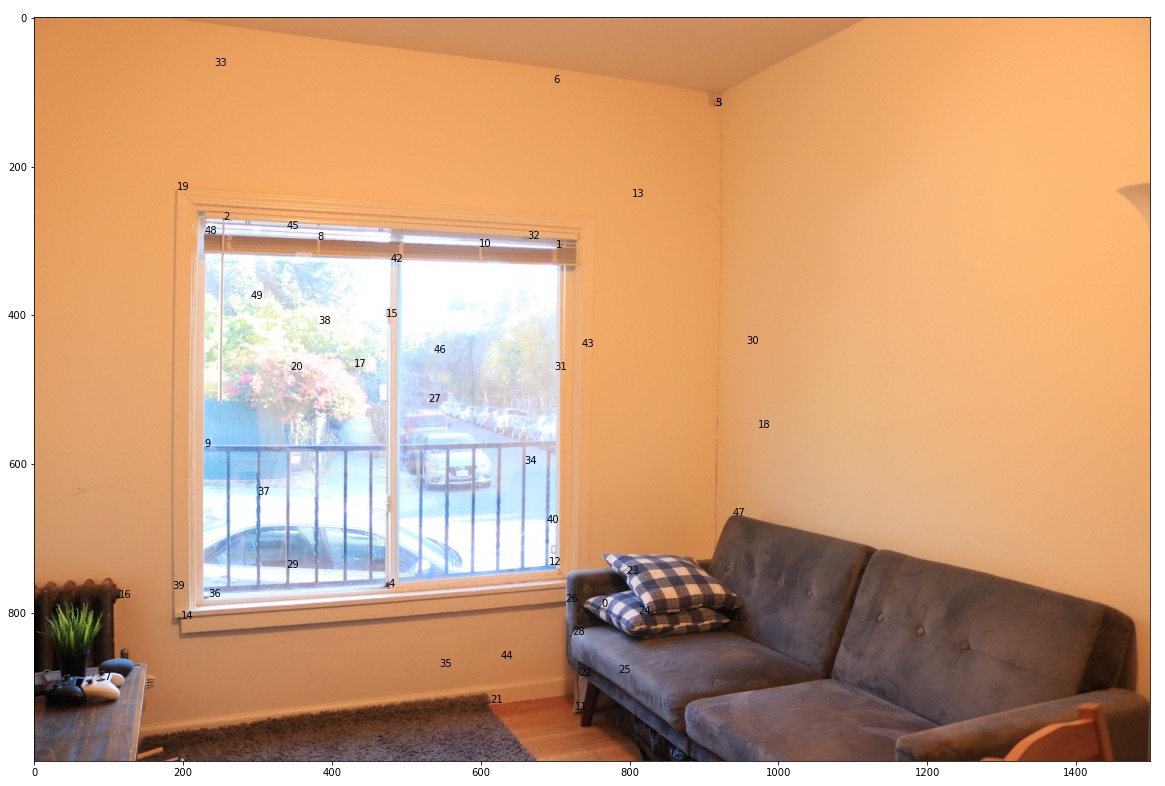
Below, the defined correspondences can be seen in all 3 images (they were identified as 4 corners of 2 windows present
in all the images) and these were collected using ginput. Then, the parameters of the homography were recovered using
the system of equations explained above.

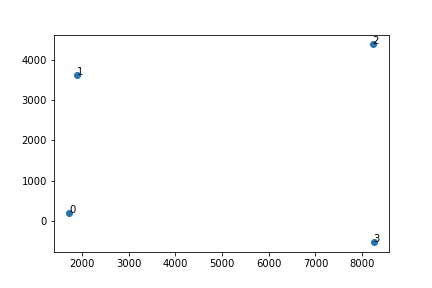
To warp the images, I first defined a find_bounds function that takes in an image and a Homography matrix and then
does a matrix multiplication between H and the 4 corners of the original image. It then divides each (wx,wy, w) coordinate in the result
by the 3rd value (i.e. the w) to bring it back into 2D. Between these 4 new coordinates, I found the y_max and the x_max value
and initialized the dimensions of the warped image to x_max, y_max.
To fill in this new warped image, I used inverse warping - Effectively taking the indices of the new image, multiplying
them by the inverse of H to find the coordinates in the original image, and then using cv2.remap to sample the pixel
values from the original image and bring them to the new, warped image. During this process, I had to make sure
all (x, y) coords before being multiplied by H^(-1) had a 3rd dimension 1 value (for the homogenous coordinate), and that
after multiplying by H^(-1), I was rescaling by w each time.
Note: For both the boundary calculation and the inverse warping, an H matrix had to be used and this was computed using the
function explained in the previous section.
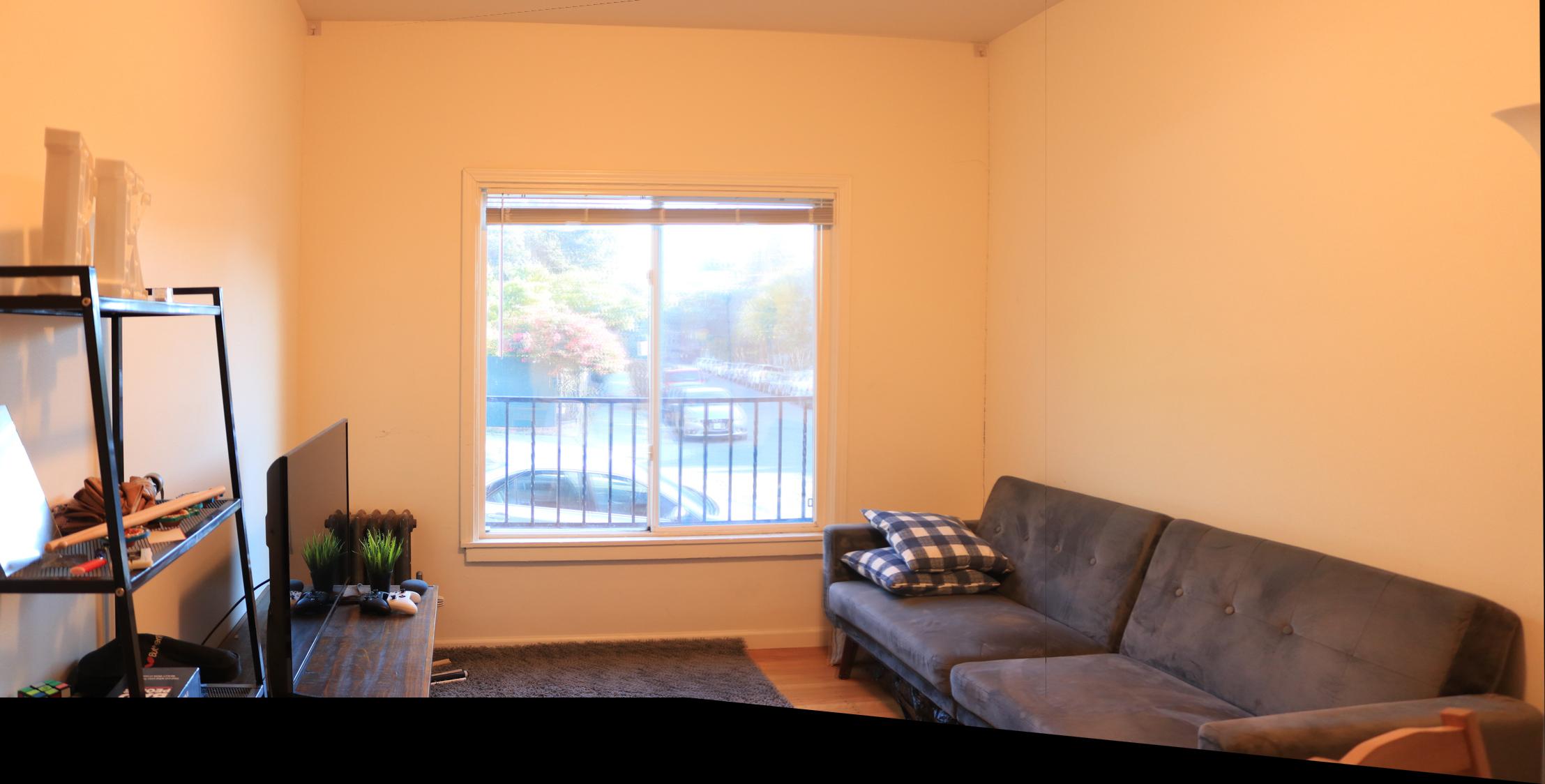
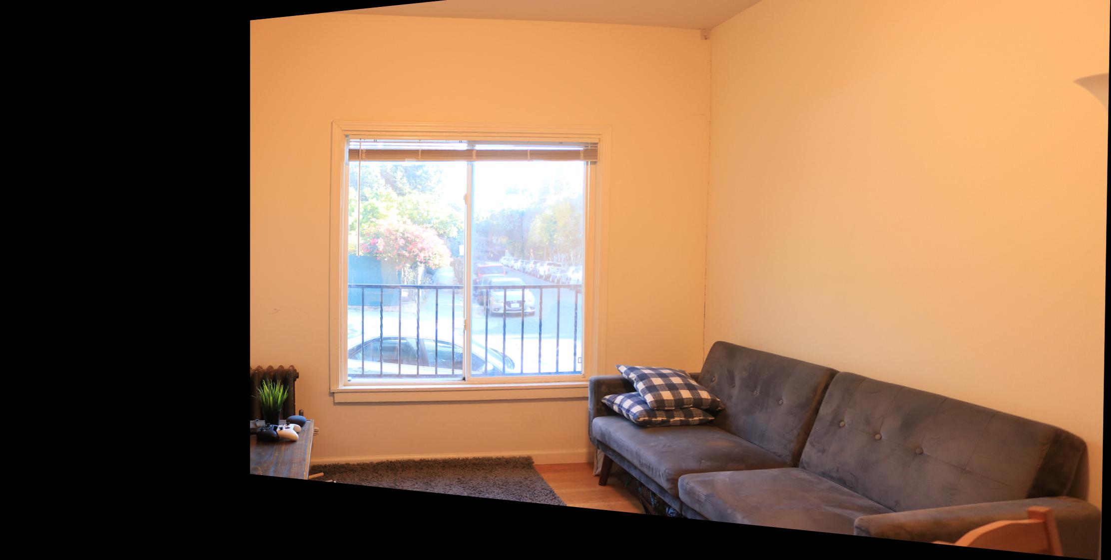
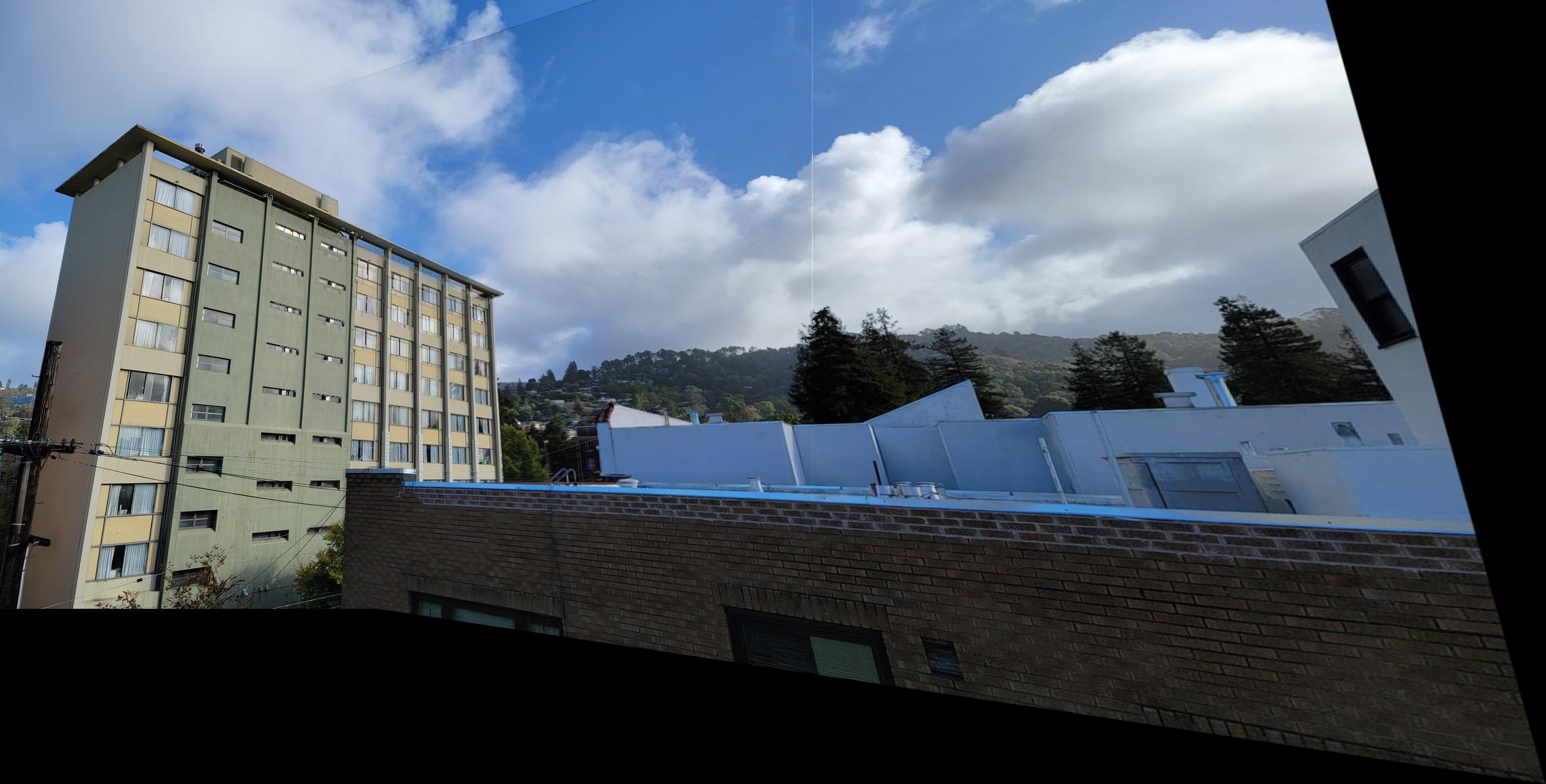
Below, you can see the results of warping the middle image into the shape of the left one, and warping the right image
into the shape of the middle one:
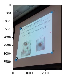
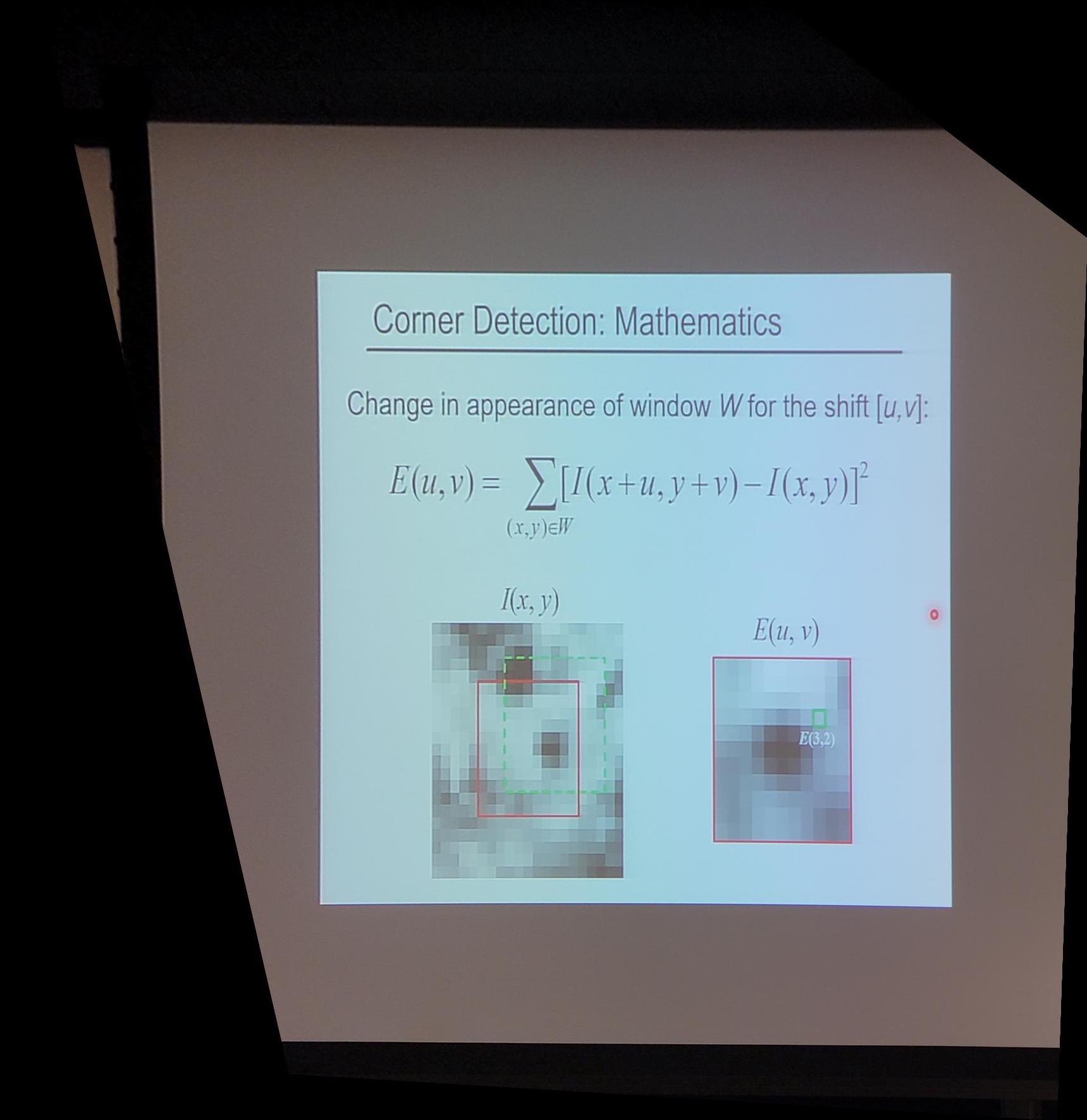
Once we have the warp algorithm working from the previous part, rectifying images becomes fairly similar. For this part, I took photos of square objects from an angle and then set the correspondence points as the 4 corners of the squares. Then I 'rectified' them by defining the 4 points of a perfect square and then warping the angled images to this square. Results can be seen below and generally show that the warping algorithm is working successfully!
To blend the images into a mosaic, I defined a function that takes in 2 images (one of which has presumably been
warped into the other's projection as explained in part 2). This function first finds the size of the mosaic by
finding the x-max and y-max between both images, and then creates two blank images with this new shape. It fills
the first blank image with input_image1 and the second blank image with input_image2. It then finds the overlapping
coordinates between these two images by checking the indices where both images are non-zero. Since we're doing a
horizontal blend here, I found the minimum and maximum x coordinates of the overlapping area, and then defined a
mask - a numpy linspace over this range (ranges from 1 to 0), which essentially acts as an alpha transition. The first image's
overlapping area is multiplied by the mask and the second image's overlapping area is multipled by (1-mask). The
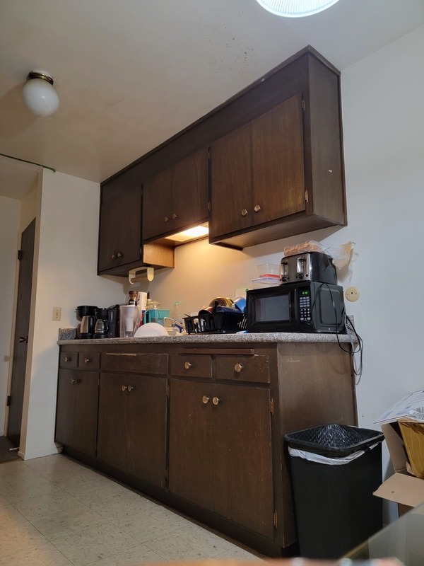
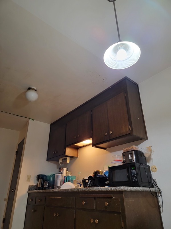
two images are then added together to create the final mosaic. Three examples of this algorithm can be seen below:
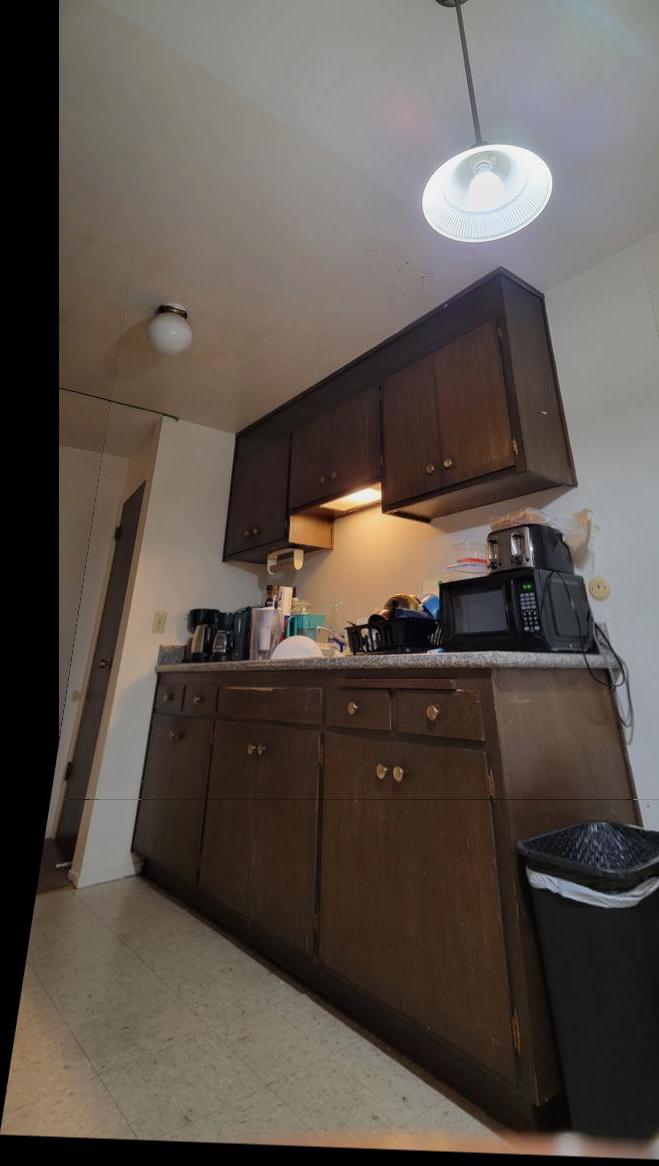
You can see with the outdoor scene of Unit 2, there is some ghosting issues because the trees and the wires move
around a little due to the wind and even with well defined correspondences, this will lead to some issues. On the
other hand, with the desk and the indoor house scene, these are a lot more stationary, so the resulting mosaic is a
lot better looking!
The most important thing I learned from this project was the new issues to keep in mind as we move from
affine triangle warps (in the last project) to projective rectangular transformations in this project. I initially
thought that the process would be quite similar and although the idea of defining correspondences and inverse warping
is still present, there were new issues I had to deal with: What if after warping, the new boundaries go into negative
coordinates? How can we rearrange the system of equations so that we can solve them even without explicitly knowing w
in the p' point? Therefore, I was able to learn the differences between projective and affine warps more clearly
by seeing the impact in the transformations themselves.
The coolest part of this project was that I've always wondered how document-scanning apps always work so well - They
allow the user to take a photograph of a document at a slight angle, identify the 4 corners of the document, and then
return an image that looks like it was scanned by an actual scanner. After working on the 'Rectifying Images' part of this
project, I now realize how the user setting the 4 points of the document is basically us identifying the correspondences
so they can warp the image into a rectangular!
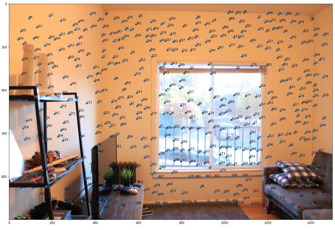
To detect the corner features in an image, I used the provided code for the Harris corner detector algorithm. The only change I made to the provided function was take in an argument for the minimal allowed distance between separating peaks so that I could use this to control how many Harris corners are generated. Below, is a figure of the Harris corners overlaid on one of the images of my living room that will eventually be used for the final mosaic.
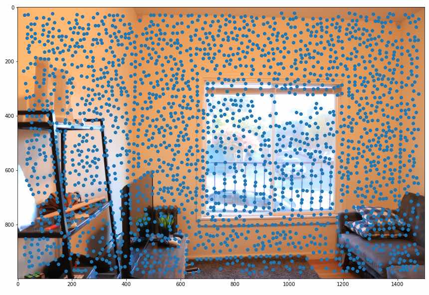
As can be seen from the above image, there's too many Harris Corners so we want to restrict the number of interest points for the image while maintaining these points are distributed throughout the image. To do this, we only retain points that have the maximum corner strength within a radius of r pixels. The formula to find these radii, as listed in the paper is as follows:

I set c_robust to 0.9, which was the optimal value according to the MOPS paper, found 500 radii values using the above formula and then, for the best corner points, I selected the 500 points that yielded those radii. You can see the 500 chosen interest points overlaid on the image.
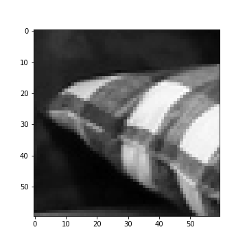
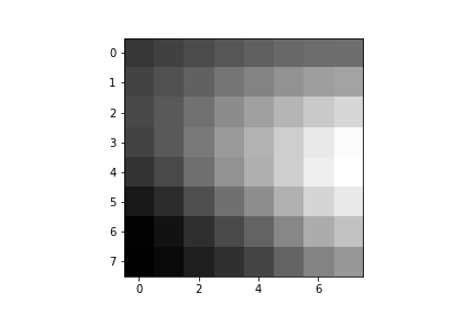
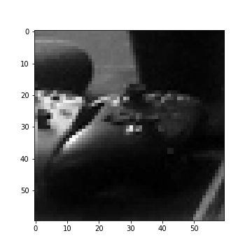
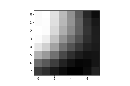
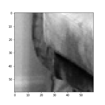
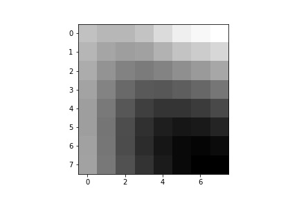
To eventually be able to match corner points between 2 different images for the mosaic, we need to have an axis-aligned feature descriptor for each of the selected points. To do this, I first blurred the image using a Gaussian filter (I found a kernel size of 30 and sigma value of 15 to be suitable). I then found a 40x40 patch around each of the interest points (from the previous section) and downsampled this to 8x8 by using a spacing of 5 pixels between samples. After sampling, I normalized the patch by demeaning it and dividing by the standard deviation. Below you can see some of the patches from the image and their corresponding feature descriptor. Note that the left are displayed as 60x60 pixels just so it's easier for the viewer to see where they come from in the overall image but the actual sampling was on a 40x40 patch.
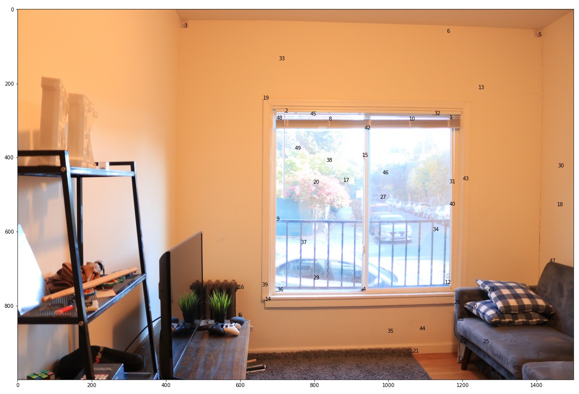
For feature matching, I first computed a matrix of SSD values where the (i,j)-th entry represents the SSD value for the i-th feature-descriptor in the first image and the j-th feature descriptor in the second image. For each of the n points in the first image, I find the first nearest neighbour and the second nearest neighbor (by indexing into the pre-computed SSD matrix), and find the ratio 1-NN/2-NN error. If this value is less than 0.25, then that point and its nearest neighbor are kept as matching features. Doing this over all points gives back the matched points, which are numbered in the two images below.
In the previous section, 50 matching points were found and through a visual check, we can see that most of them do seem to be correct correspondences. However, even a single outlier can affect a homography calculation which is why I then use RANSAC to compute a robust homography estimate. To do this, I randomly choose 4 matching points between the images, compute the homography matrix H from the 4 points in image1 to the 4 points in image2 (using the computeH function written in part A of this project). I then check the number of inliers for this homography as follows: Warp all the remaining points in image1 and count which ones are within some epsilon of their match in image2. Whichever transformation has the most inliers is chosen, and then I recompute H using all the inliers for a more accurate estimate. I used an epsilon value of 5 and 20,000 iterations for the above images of my living room. Below, I have compared the warp result using RANSAC to the warp result from the manually marked correspondences in part A.

The fact that these are very similar is a good sign indicating the RANSAC algorithm is working as expected! Next, we can create the actual mosaic.
To create the final mosaic, we can put together all the steps from above as follows:
1. Find the Harris corners for both images using the provided code, and then use adaptive non-maximal suppression to restrict these
to 500 interest points in both images.
2. Extract a feature descriptor for each of the 500 points in both images by first blurring the image, taking a 40x40 patch around
the interest point, and then downsampling to 8x8.
3. Match points between the two images by checking the (1-NN)/(2-NN) error ratio (using SSD as the matching metric)
for each of the points in image1 (arbitrarily) and only accepting matches that have a ratio < chosen epsilon.
4. Use RANSAC to repeatedly select 4 points at random from the matching points, compute the homography matrix, check the number of inliers
and repeat this process 20,000 times. Then take the argmax over the number of inliners, and recompute H using all inliers this time.
5. Warp image2 into the projection of image1 using the H found in step 4.
6. Use the alpha blend algorithm (created in part A) to combine the two images to create the final mosaic.
Below, you can see an example of this process being used to create a mosaic for the living room photos (used throughout this section)

We can also compare the mosaic generated using the manually labeled correspondences and the mosaic that was made with automatic feature detection and matching. Once again, the results are extremely similar and I would say that both panoramas are fairly pleasing to the eye. I would argue that the auto-generated one is slightly better in the middle, overlapping region where (after zooming in), we can see the manually labeled one is a little blurrier outside the window and near the window's borders. This is probably because the manually labeled one relied on me clicking on the correspondences and if I missed by a few pixels, it would lead to slight misalignments and blur.
Some other generated mosaics using this same automatic process:
From this whole project and the paper we were implementing, I found the idea of using the 1-NN/2-NN error as a test to be the coolest part. It is a very simplistic idea and yet, it makes a lot of sense both mathematically and from a practical sense: Don't go with either suitor if it's too difficult to choose between them! This also made it really efficient to check for outliers without any visual input from the user. Overall, I really enjoyed this project because it definitely made me appreciate how much work my phone has to do everytime I take a panorama (clearly something I had been taking for granted)!