Justin D. Norman Project 4 Part 1

The goal of this project is to demonstrate the foundational principles of image warping through the applied technique of image mosaicing. Creating a mosaic involves several steps on two or more images:

• Registration
• Projective Warping
• Resampling
• Compositing

1. Shoot and Digitize the Pictures

2. Recover homographies

The next step was to select the keypoints and (and store them for the many future iterations of the image pipeline). I used some of my learning from previous projects to write a ginput() UI, the results of which are below:

From here, I was ready to recover the the homographies, which involves the following transformation p’=Hp, where H is a 3x3 matrix with 8 degrees of freedom.

I implemented this by creating a function computeH(im1_pts, im2_pts) which sets up a linear system of n equations (i.e. a matrix equation of the form Ah=b where h is a vector holding the 8 unknown entries of H)

3. Warp the images

From here, I implemented a function warper(im, width, height, H) which uses the parameters of the homography to warp the images into thier new form. I used the input parameters height and width to set the size of the new image. The result is below for the first image:

...and for the second

4. Blend images into a mosaic

Now that I have the two individual warped images, I chose to blend them two together (rather than simply add them up) to minimize the edge artifacts as much as possible. I used the weighted alpha/beta blend technique which definitely did not produce as ideal of an result as I was expecting. There's some ghosting for sure and lots of edge artifacts.

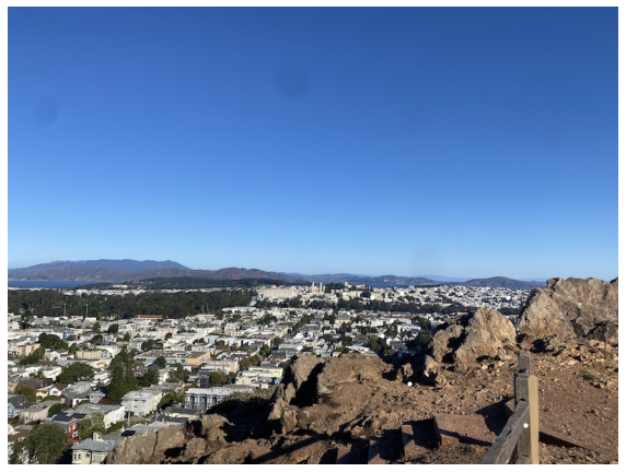
Here is another example from the other side of the hill

Overall I learned:

• I still have some gaps in my knowledge about blending--I tried to create a Laplacian blend and couldn't get it to work
• Keeping track of image size and relative position is critical in this kind of work
• Setting up systems of equations in code is simple, but is not easy at all to execute conceptually

Justin D. Norman Project 4 Part 2

The overall goal of the 2nd part of the project is to is to create a system for automatically stitching images into a mosaic. A secondary goal is to learn how to read and implement a research paper. The steps involved in this process are:

• Detecting corner features in an image
• Extracting a Feature Descriptor for each feature point
• Matching these feature descriptors between two images
• Use a robust method (RANSAC) to compute a homography
• Proceed as in the first part to produce three mosaics

2.1 Detecting corner features in an image

2.1.1 Start with Harris Interest Point Detector

Detecting corners was a simple enough task to do with the given get_harris_corners function that was provided. The results of those detections with a min distance set by parameter are below.

2.1.2 Implement Adaptive Non-Maximal Supression

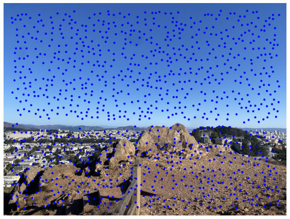
Even with a higher minimum distance, it's still necessary to restrict most of the points returned by the corner detector. This is the function of ANMS in this project. I chose to use 400 interest points as an input parameter to the calculation and a c (or subpression radius of 0.9). The implementation was adapted from Brown et. al's Multi-Image Matching using Multi-Scale Oriented Patches.

2.2 Extracting a Feature Descriptor for each feature point

2.2.1 Implement Feature Descriptor extraction

Using the Harris/ANMS corner points, we can now shift focus to extrating the feature descriptors for each of the points in order to setup the feature matching step. This is accomplished by selecting a 40x40 sample centered at the each point, blurring that sample using a gaussian, and then resizing it to a 8x8 segment know referred to as a feature descriptor.

2.2.2 Implement Feature Matching

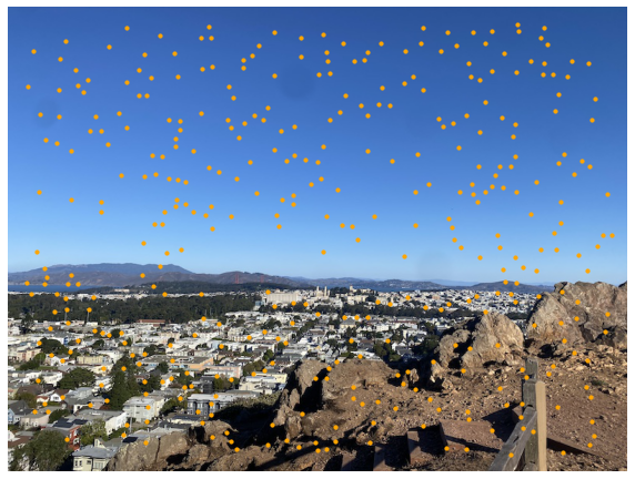
As stated before, these feature descriptors were then used to further restrict the number of points. The SSD is computed between each pair of corresponding feature descriptors, and only pick the best (and second best) matches. Those are displayed below.

2.2.3 Use a robust method (RANSAC) to compute a homography

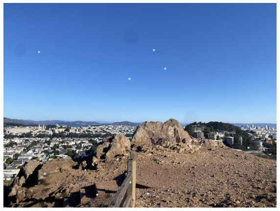
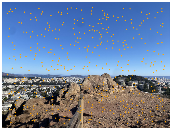
Let's Keep reducing. RANSAC is a simple algorithm that works quite well. The idea is to select randomly 4 points and then to compute a homography and perform a check to determine the degree to which other points form a "consensus" with the homography. Every time through the algorithm if the consensus points are better matches than the previous steps, these are selected as the new best. 1000 iterations are selected in this implementation and a very consistent set of points are selected. The results are below.

2.3 Proceed as in the first part to produce a mosaic

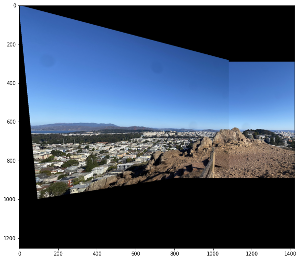
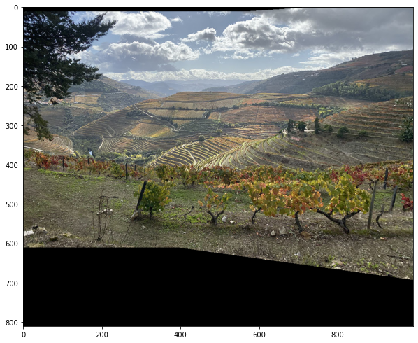
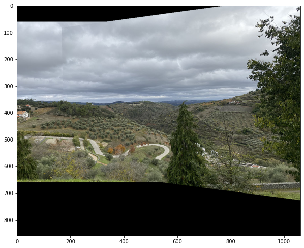
The final step was to stitch together the images and then also blend them into a mosaic. Here are the results from 3 image pairs taken all the way through the pipeline. The first is the two images I took on tank hill. The second and third pair are taken as accidental inputs to a panorama while I was on a motorcycle trip in Portugal just prior to the COVID-19 pandemic.