Project 4: Image Warping and Mosaicing

CS194-26: Image Manipulation and Computational Photography

Author: Sunny Shen

Part A

Overview

In Part A of this project, I took a bunch of photos of objects/scenes from different perspectives. I calculated the homography and did projective transforms on them, and then I stitched & blended the images together to create panoramas.

1. Recover Homographies

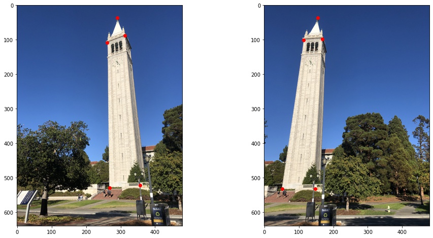
Before doing all the cool warping and projective transformation, we need to find key points in images and calculate the homography matrix that warps the images onto each other.

Homography matrix H is a 3x3 matrix with 8 degrees of freedom, and we transform keypoints p in th source image to the destination images key point p' based on H: p’=Hp.

To solve for H, I set up a linear system of n equations (Ah=b where h is a vector holding the 8 unknown entries of H).

image source

2. Warp the Images

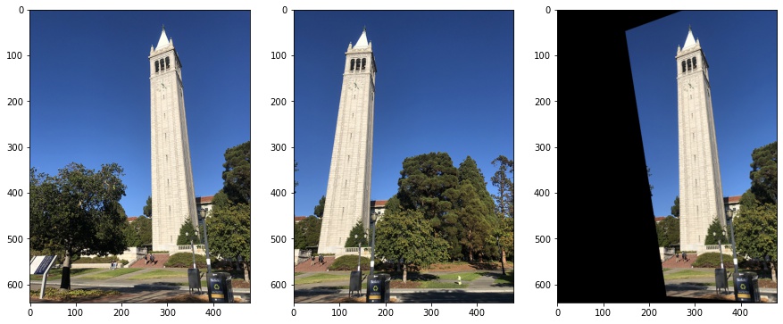
Now with the homography, we can warp the image with the projective transformation! Note that if the output image is the same size as the original image, we will "lose" part of the image after projective transformation because we not only change the shape defined by the key points but also the location -- so we need to change the output image size to retain most information in the image. Also note that there are a lot of black pixels in the warped images, and that is because there is no information available in those pixels.

3. Image Rectification

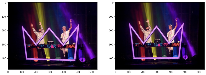
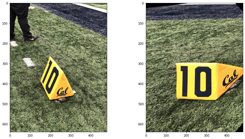
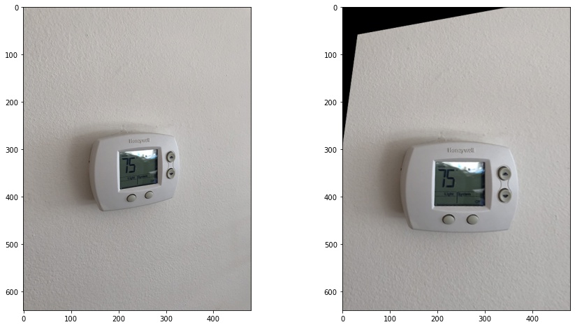
Let's rectify some images that we know some ground truth of the objects -- for example, we know that from a different perspective the objects are supposed to be 'rectangular'. And we use the rectangular shape as 'target' and warp the original images into that shape. Here are a few examples!

4. Blend the images into a mosaic

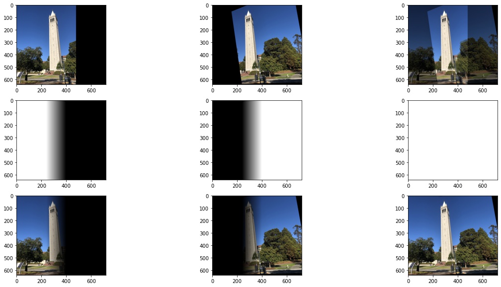
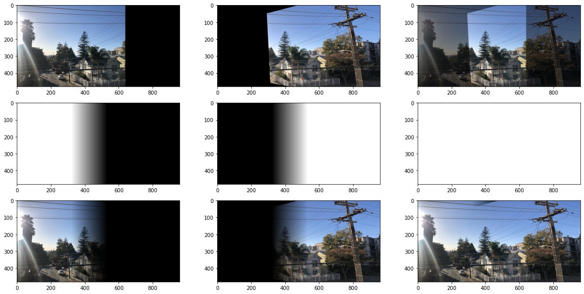
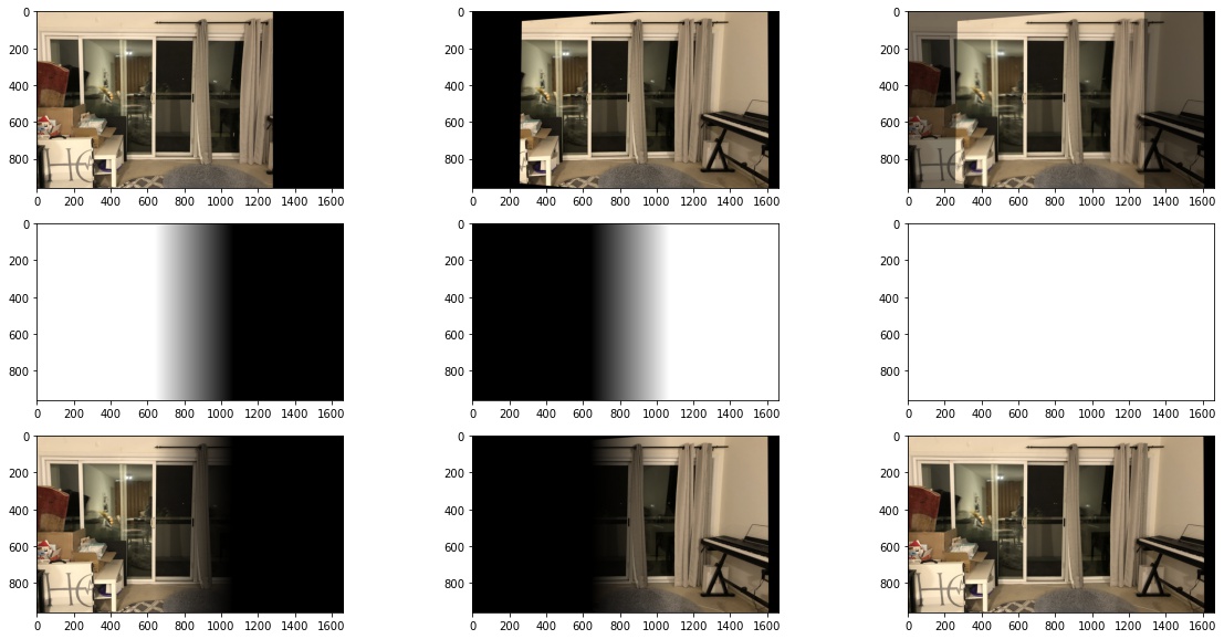
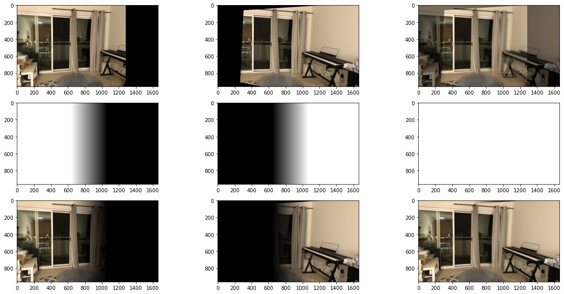
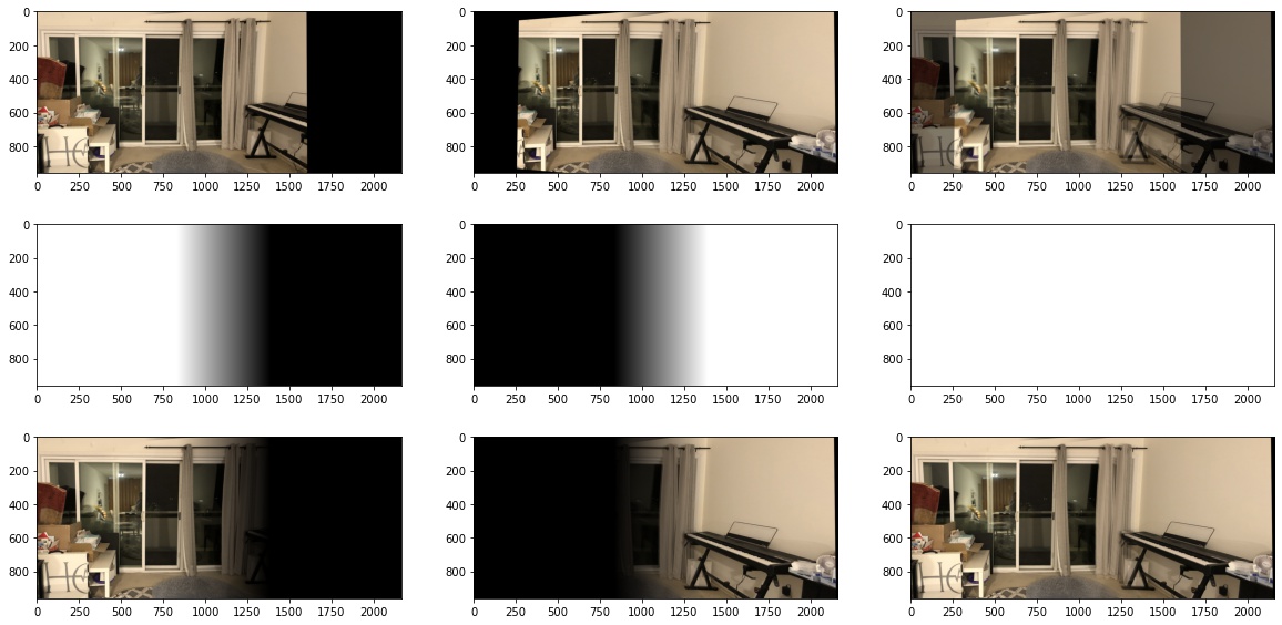
Let's create some panoramic pics! After applying projective transformations, we need to find a way to combine and blend all the images together. Simply doing img10.5 + img20.5 will create weird edges at the intersection of the images. But alpha blending -- Create a gradient mask that linearly decreases/increases the weights from 1 to 0 (or 0 to 1) for parts that overlap -- help the images blend well.

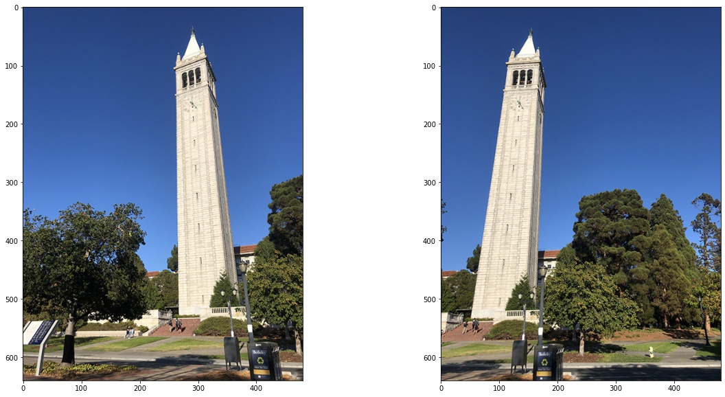
Example 1: Campanile

Originals:

Mosaicing in Progress:

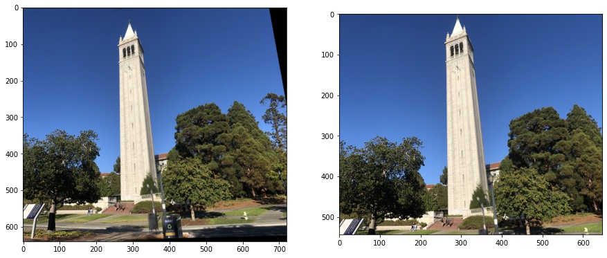
Final output (before and after cropping out black parts):

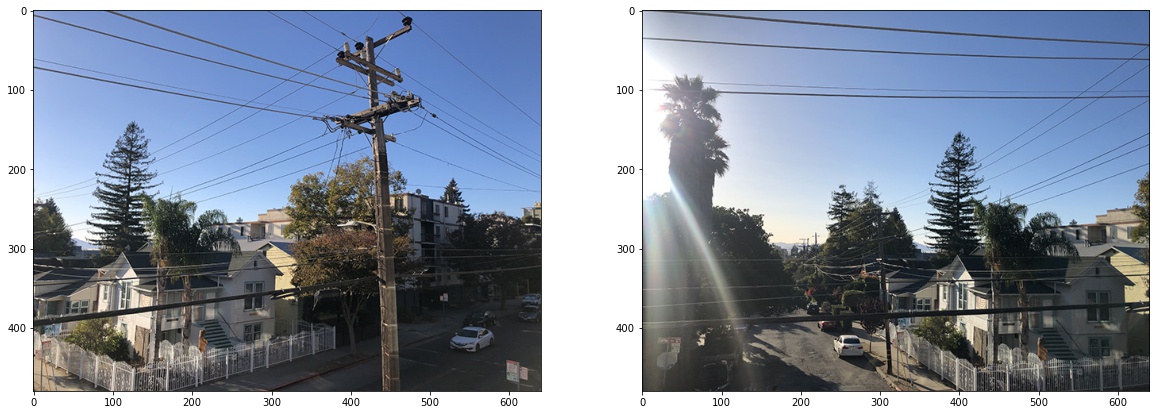
Example 2: Street View

Originals:

Mosaicing in Progress:

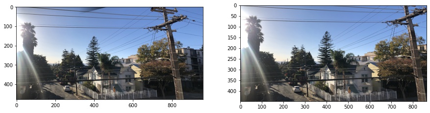
Final output (before and after cropping out black parts):

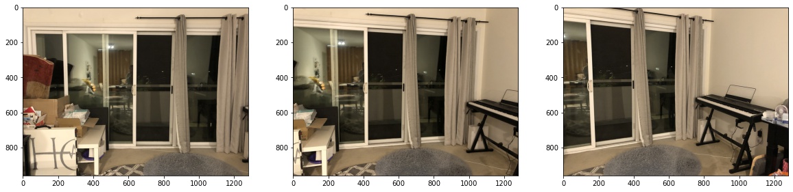
Example 3: Living Room

Originals:

Mosaicing in Progress:

1. Warp the mid pic & blend with the left one

1. Warp the right pic & blend with the mid one

1. Blend the 2 panoramas to 1 full panorama

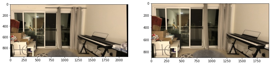
Final output (before and after cropping out black parts):

What's the most important/coolest thing I have learned from this part?

I think it was super cool to apply projective transformations to images and think about how to blend them together. I took most photos from my phone, and my eyes weren't able to tell that the color/lighting/other specs of the camera slightly changed when I take 1 photo from 1 perspective and take another photo from a different perspective. I was trying to warp and blend some sunset photos from phone and I realized that the color of the sky didn't exactly match. I didn't put those examples on the website but I think it was cool to learn about that.

Part B: Feature Matching for Autostitching

In Part A, I did feature matching manually by clicking on key points on images, which is a lot of manual work and the result can be significantly different if my clicks are a few pixels off from where I meant to click.

In Part B, I implemented the feature detection algorithm outlined in the paper "Multi-Image Matching using Multi-Scale Oriented Patches" to generate panoramas.

Step 1: Harris Interest Point Detector

First, I find points of interests with the Harris corner method. The threshold I used was the Average of corner strength - SD of corner strength. That seems to give a good amount of harris corners.

Step 2: Adaptive Non-Maximal Suppression

One naive way to select "good" interests points may be to choose the ones with biggest corner strengths, yet those interests points tend to cluster around the same area and do not necessarily represent all the edges/corners well -- in this case, an overwhelming amount of points are among the trees which may not be that helpful for projective transoformation

ANMS allows to choose points that are both helpful and nicely spread out in the whole image. I calculated the impression radius of every single interest point based on the following formula:

where I is the set of interests points and x_i is 1 point -- Here, I set c_robust = 0.9, just as the paper. Here's the result of choosing 500 points with ANMS:

Step 3: Feature Descriptor Extraction + Feature Matching

Now we have some "good points" on each image, we need to figure out how to match them on both images.

Feature Extraction - At each interest point, we sample a 8x8 patch from a 40x40 window and then normalize them.

Feature Matching - We then use these normalized patches to calculate the 2 nearest neighbors of each patch from image A from all patches from image B. If the best NN has significantly lower distance (measured by SSD) than the 2nd NN, then it's a good match. More specifically, it's a good match if SSD_1NN / SSD_2NN < threshold (I used 0.4 by default, but sometimes increasing the value gives better results too)

Step 4: RANSAC

As we can see from the matches above, (unfortunately) not all the matches are correct. To compute the homography, we have to have accurate matching points and we pretty much have 0 tolerance of making mistakes there. Therefore, we use RANSAC to find the best possible homography. RANSAC works as follows:

Repeat the following:

1. Randomly sample 4 matching features
2. Compute the homography
3. Use the homography to find inliners where the predicted pixel location after projective transformation is very close to the expected pixel location -- find the number of inliners

Then, we keep the largest set of inliners and use them to recompute H

In my experiments, I found that doing 1000 iterations gave pretty good results.

Finally, the Panorama!

I compare the panaromas created by auto-feature detection and manual feature selection -- turns out the auto feature detection has slightly better results!

Example 1: Campanile

Originals:

Auto-stitching:

Manual: (slightly blurrier than auto)

Example 2: Street view Pano

Originals

Auto Feature Detection:

Manual:

Example 3: Living Room Pano

Originals:

Auto-stitching:

Manual: (the edge of the piano is blurrier than the result of auto-stitching)

What I learned (Part B)

I think the entire topic of automatic feature detection is very interesting - using Harris corners and playing with different threshold was fun. I think the most interesting part is RANSAC (what a genuis idea), and it's so powerful that if we do a large amount of iterations we are able to find the right homography even if we don't have a good set of matching interests points.