Homographies and Panoramas

I came to college to be exposed to new perspectives. Little did I know that I could just make myself a new one.

Introduction

In our last project, we got to experience the power of transformations firsthand, using them to seamlessly morph objects and faces from one to another. This time, we're going to kick it up a notch (and a point), and use homographies to transform the apparent points of view of entire images. We can use this technique to do all sorts of cool things, such as peeking at our friends' notes, and stitching together panoramas from separate pictures of a scene.

Part 1: Defining Correspondences

Just like last time, for this to work, we need to start by defining correspondences between two images (or an image and a goal). Last time, we split our images into triangles, because our affine warps were determined by three points. However, this time, because we're applying homographies across an entire image, we need four co-planar points. Then, to define our homography, we need to select the points that we want those points to be warped to in our destination image. Then, with these eight points, four from each image, we can solve for our homography by setting up a system of equations to get the coefficients of our homography matrix.

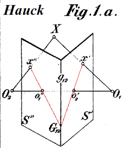
This image (stolen from this extremely helpful medium post), shows us one such way to do this:

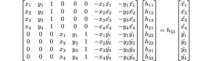
To set this up, we take the x and y coordinates of each of our points and fill them into this matrix. To make our lives a little bit easier, I switched the equations around so that the x and y coordinates of each set of corresponding points were adjacent to each other in the matrix, by basically interleaving the rows of the top half and bottom half of the A and X matrices. This allowed me to more easily iterate over points and include more than eight in the equation and reduce the noise in the calculated homography. However, by including more than eight points, we introduce the possibility of overconstraining our equation, which requires the use of least squares to solve for the best fitting homography. The Ordinary Least Squares, or OLS equation is as follows:

In this case, since we want to solve for our unknown $H$ matrix, we will use this equation as follows, where the $\vec{h}$ vector is the components of the matrix in row-major order, and $\vec{p}$ is our vector of target points, $\hat{x}_i, \hat{y}_i$:

which gives the solution:

Then, by appending a scale factor of 1 and reshaping our array, we have found our homography matrix!

Image Warping

This homography matrix allows us to calculate the transform between the camera pixels for different images taken from the same point. In doing so, it also allows us to "change" the perspective from which an image is taken, so long as we are not changing the position of the camera. This is a little confusing, so let me illustrate with an example:

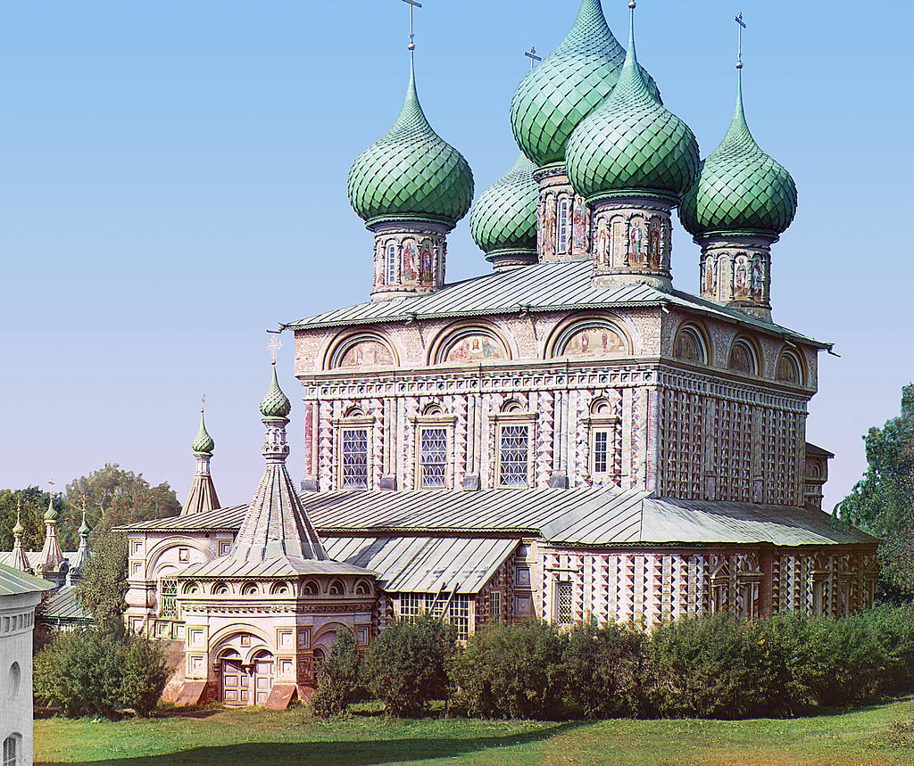
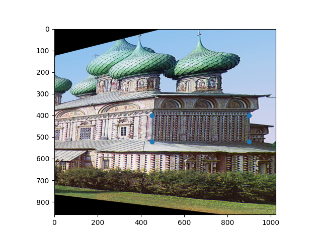
Let's take this image of the Church of the Resurrection in Kostroma. You may remember it from project one, where we got to see it turn from black and white to color miraculously before our eyes. But unfortunately, the image that Prokudin-Gorsky took of it was from a bit of a weird angle. What if we wanted a view of those gorgeous details on the side? It's not like we can go back to 1909 and take another one. So let's try using a homography!

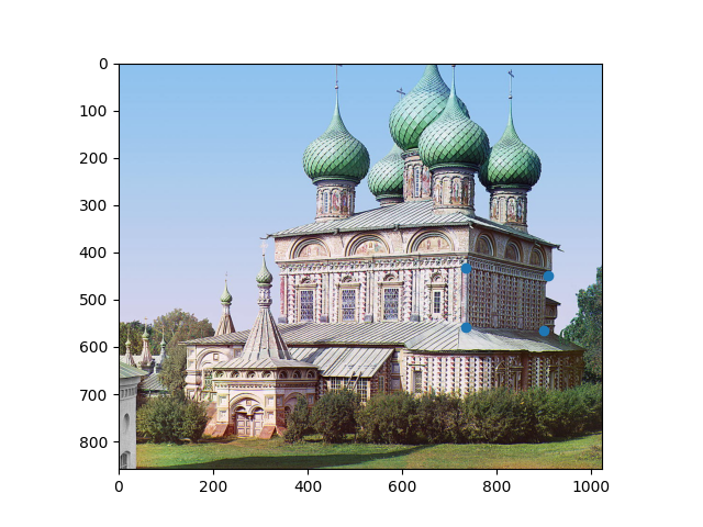
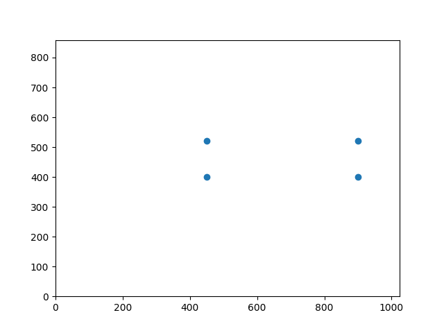
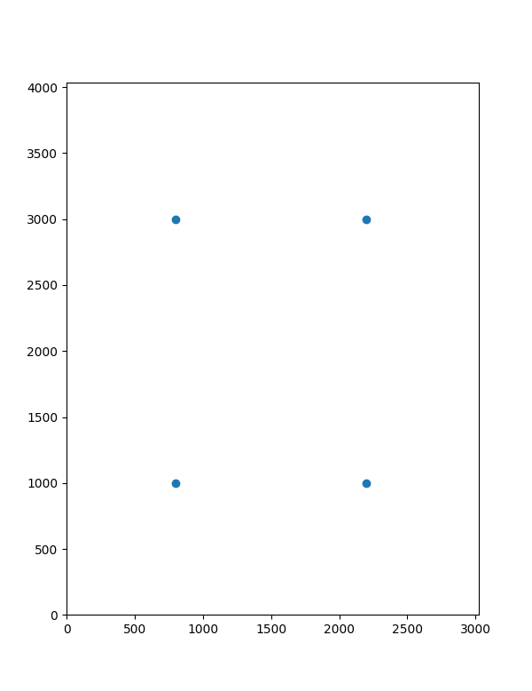
We want to "turn" the church so that we're looking at it side-on. We can do this by selecting four points on that face of the church and computing the homography from there to the rectangle that they would be if they were forward-facing:

Hmm. Well, that's a little unexpected. The side looks great, but what the heck happened to the rest of the picture?! As it turns out, this strange-looking transformation brings up two of the most interesting points about computing homographies, both of which are fundamental to understanding exactly what these computations do to an image.

First, homographies can change the perspective that an image is viewed at, but not the perspective from which it is viewed from. This means that the position of the camera relative to the objects in the scene cannot change. Because this image was taken from an angle to the far to the front and side of the church, any homography computed from it will also appear to be taken from that same position. If Prokudin-Gorsky had a distrotion-free, massively wide-angle lens, and shot this image from the same position but facing normal to the side of the church, this is how the church would appear. We can't exactly recover the way that the church would have looked from the side, because that would require moving the position from which the image was taken, and a homography cannot do that.

The second point, which is highly related, is that homographies cannot compute new information. That's why we end up with those black bars and weird distortions in the final image. Again, because we can't actually move the camera, we don't know anything except what is captured in the original image. If a point in our new perspective is beyond the borders of our original image, we're out of luck. There's simply nothing that we can do. That's why the rest of the church is still hidden behind the side wall, even though a straight-on perspective should have captured that. It's not in the original image, so it's not in our homography either.

But on objects with less depth, this approach is more effective. Let's say you're sitting on your bed, and you realize that you forgot your notes over on your desk. Sure, you could get up and go grab it, but what if you didn't have to? Homographies to the rescue!!

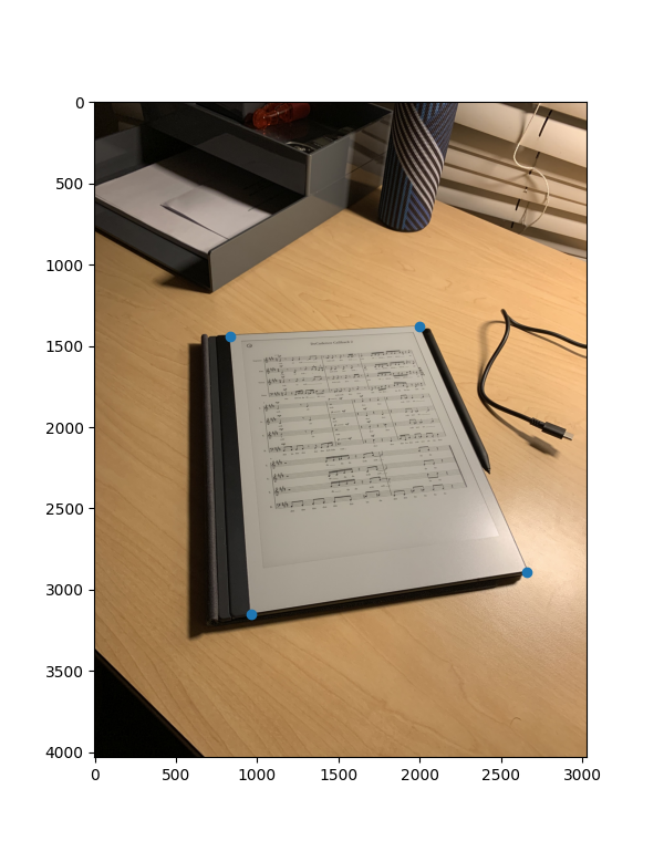
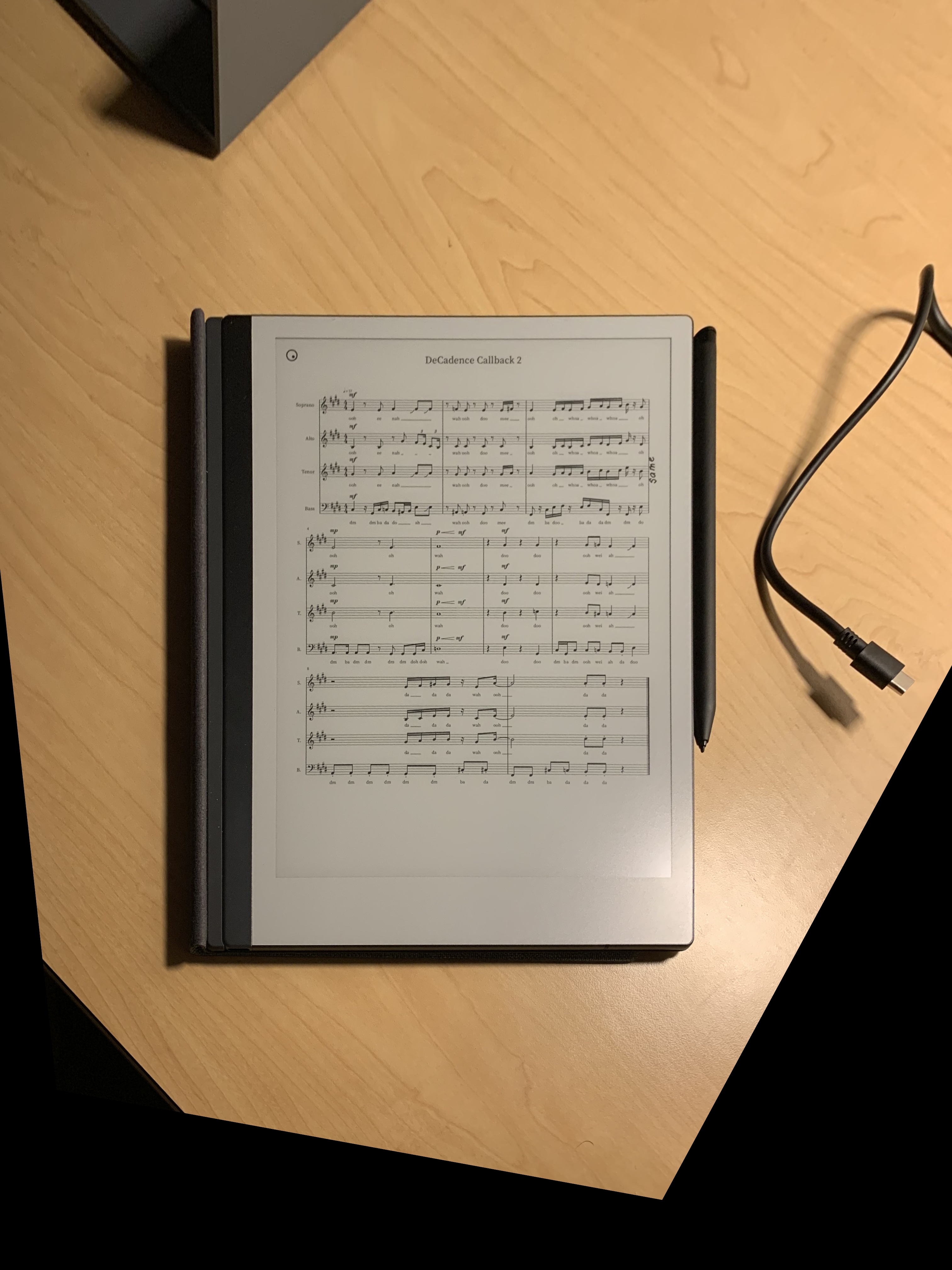
Oh, whoops. Wrong kind of notes.

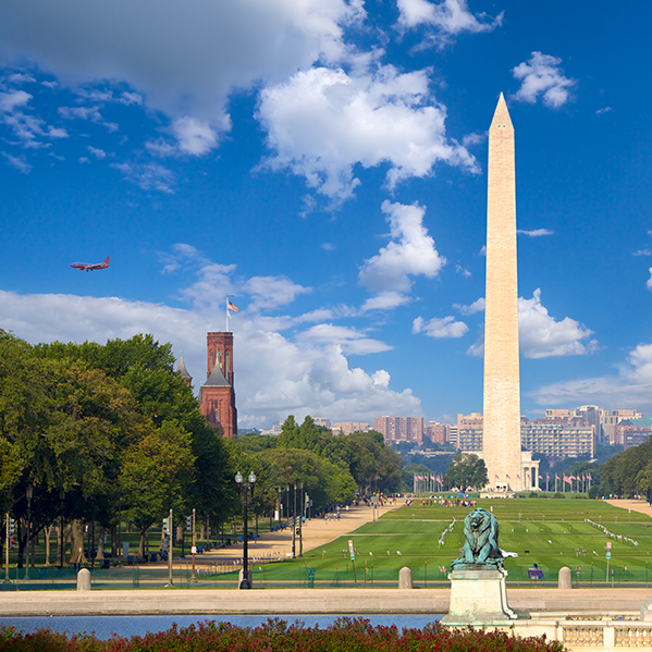
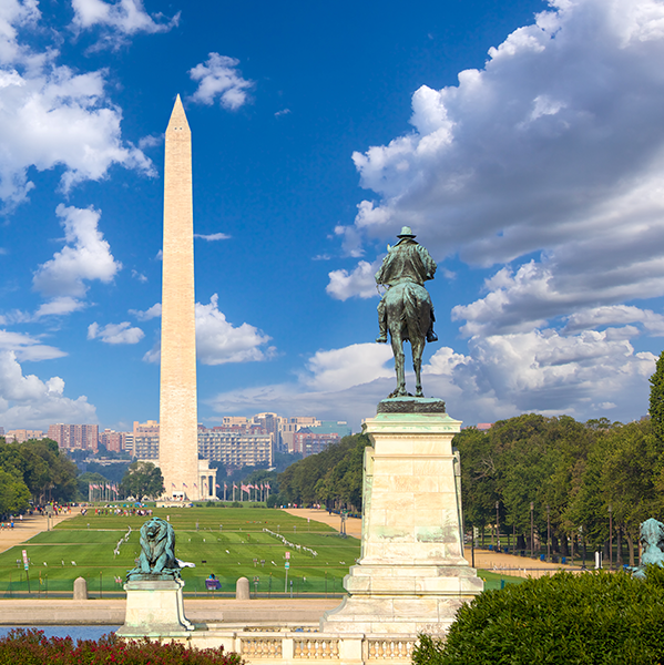
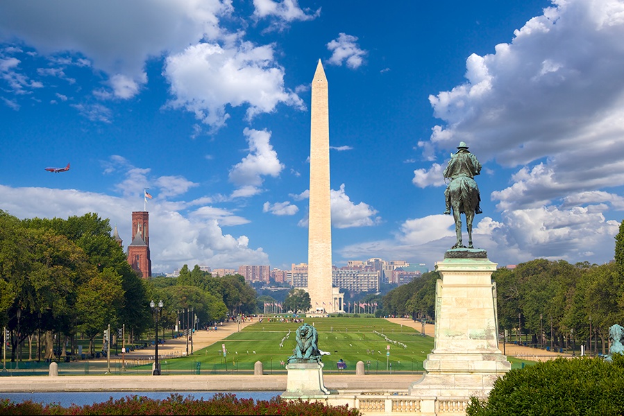
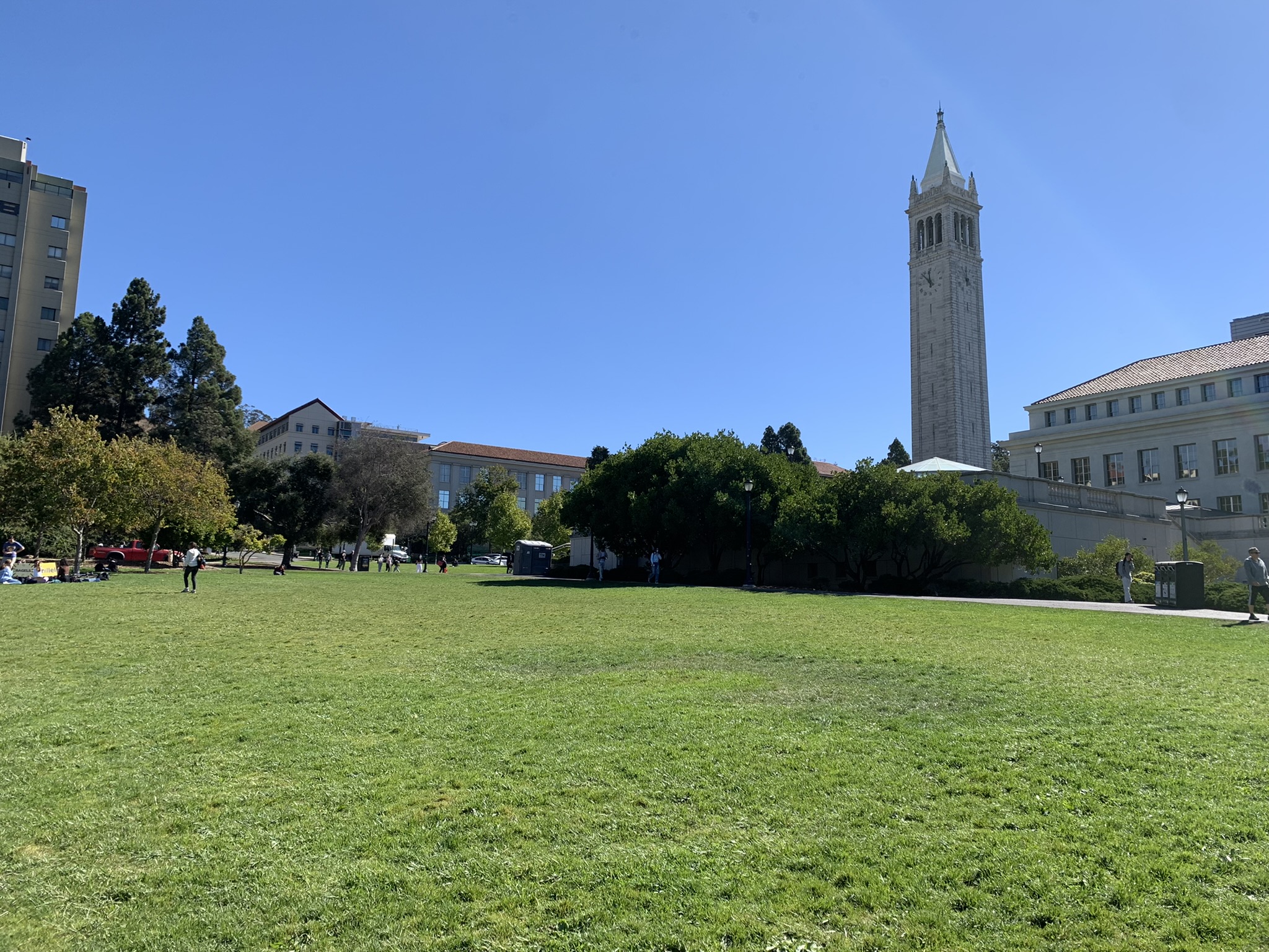
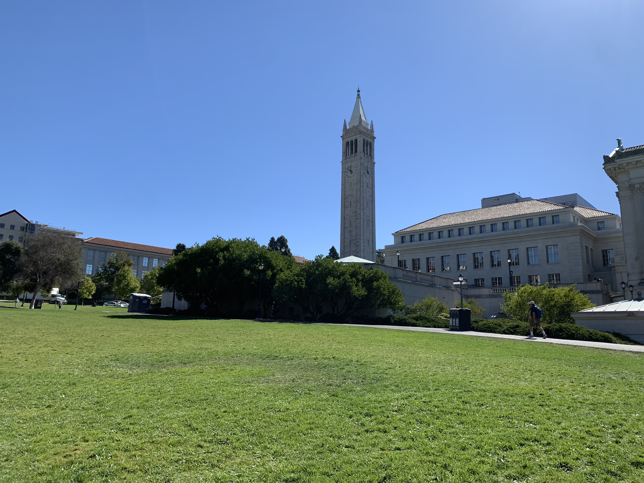
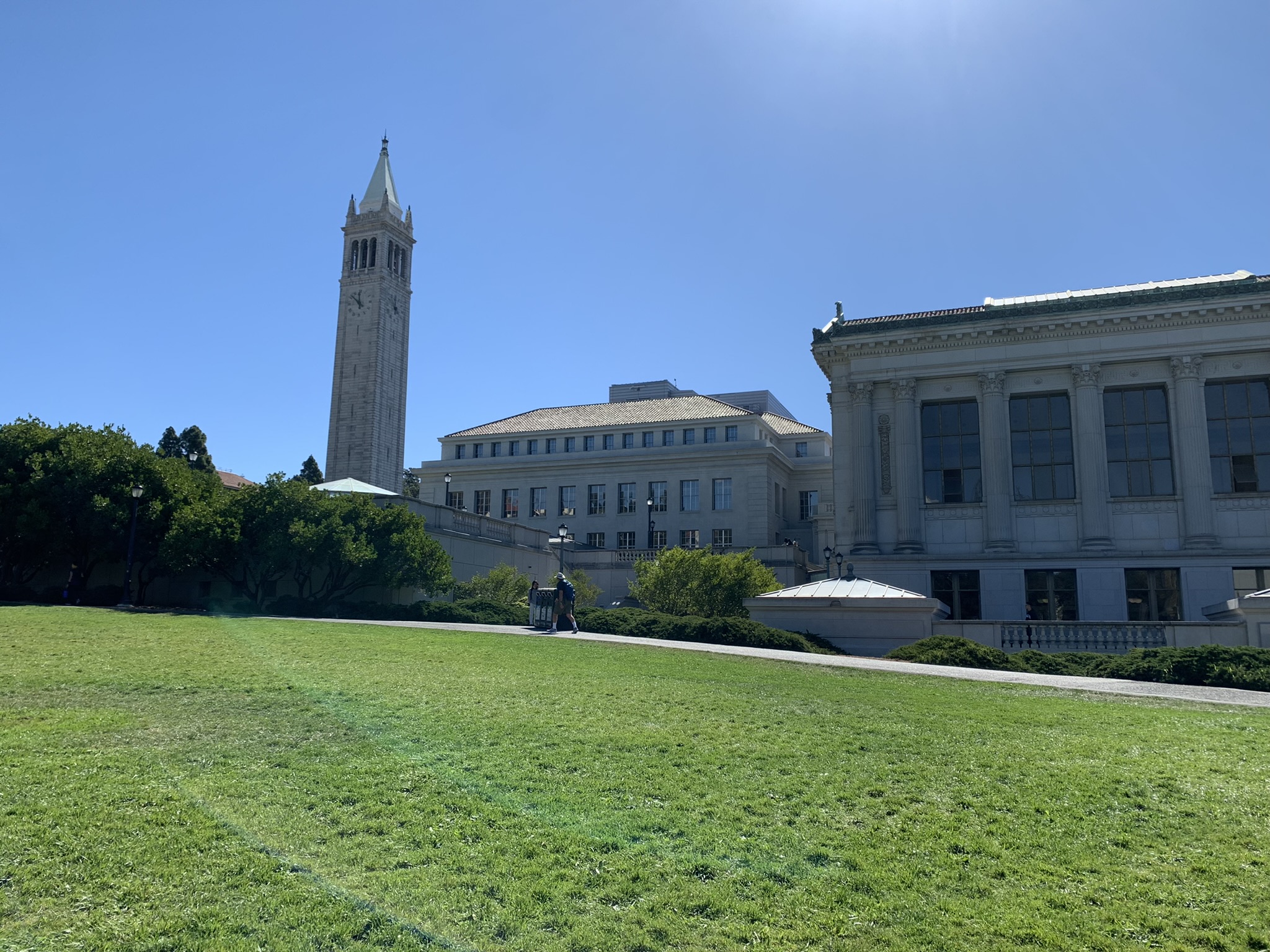
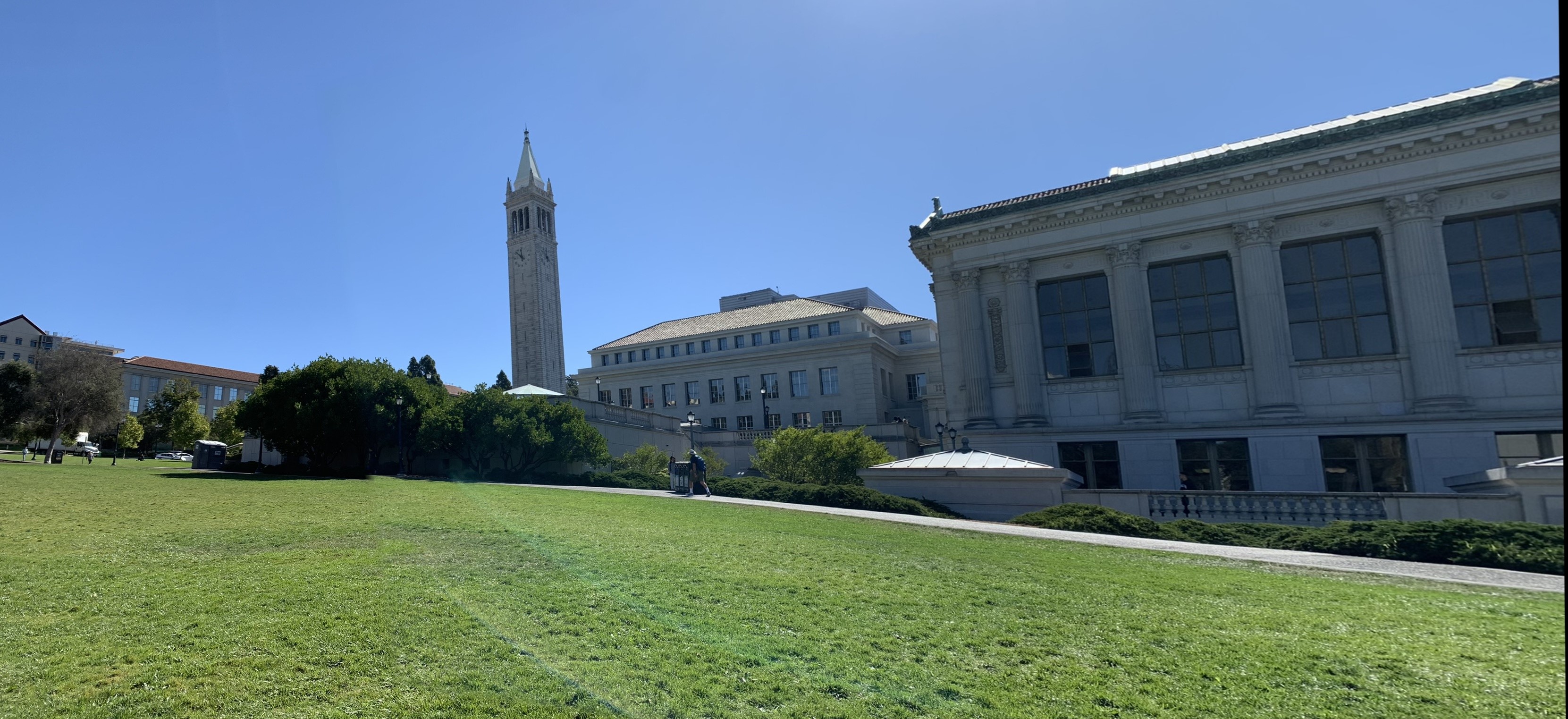
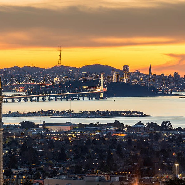
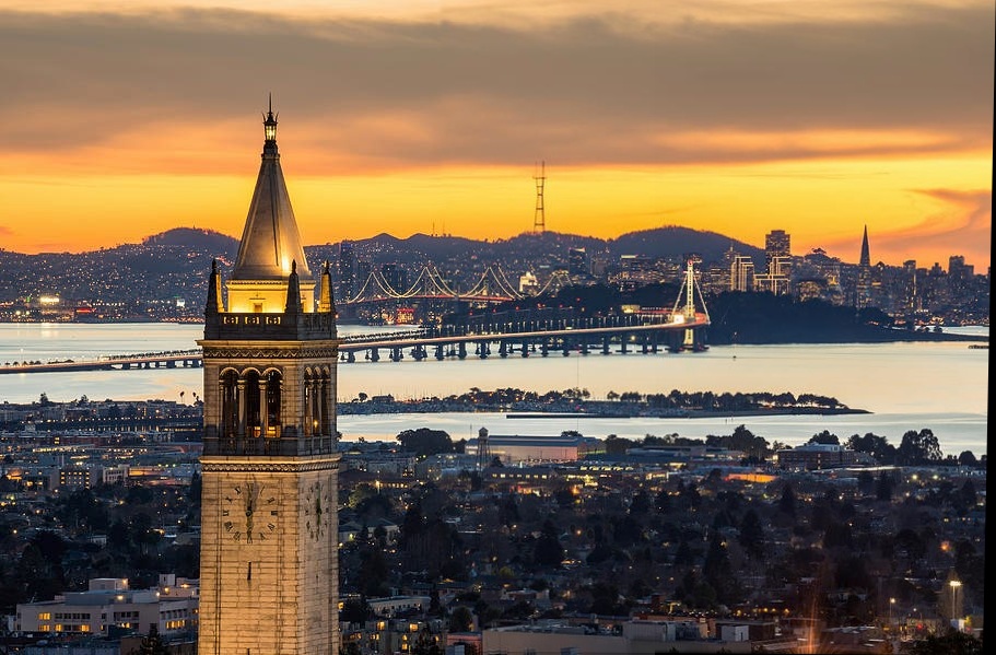
Image Mosaics

This same technique can be used to create mosaics of images. Simply use the same code to align the corresponding points in each image, add a little bit of blending, and voila! You've got a seamless mosaic!

That's all for now! Tune in next time, when we learn to remove the annoying, mistake-prone human from the process!

Letting the Robots Take Over

Now that we've gotten pretty comfortable with this whole stitching thing, let's try something radical: getting rid of the human! The most time-consuming and problematic part of the whole process is defining the points, so why don't we try shifting the responsibility to the computer??

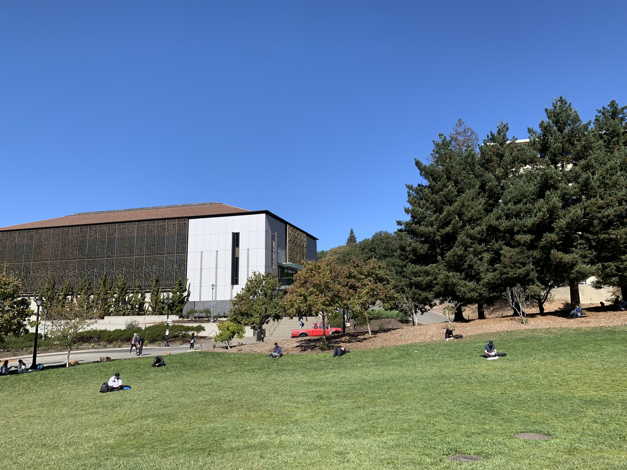
The first challenge is figuring out what points are best to match on. The best points to match are the points that will be very clearly prominent in both of the photos. But what kinds of points would those be? Obviously, they can't be the ones in the middle of places like the sky or blank walls, because they look to similar to every other point around them, but what about points along the edges of roofs or on textured surfaces? How can we tell them apart?

Well, as it turns out, there's a really obvious solution: corners. Places where there are significant changes in both the x and y directions tend to make easily identifiable and recognizable signatures, and thus also tend to look similar in all of the images of them. We can find corners using a Harris Corner Detector, which was already implemented for us in the starter code. So let's try it out!

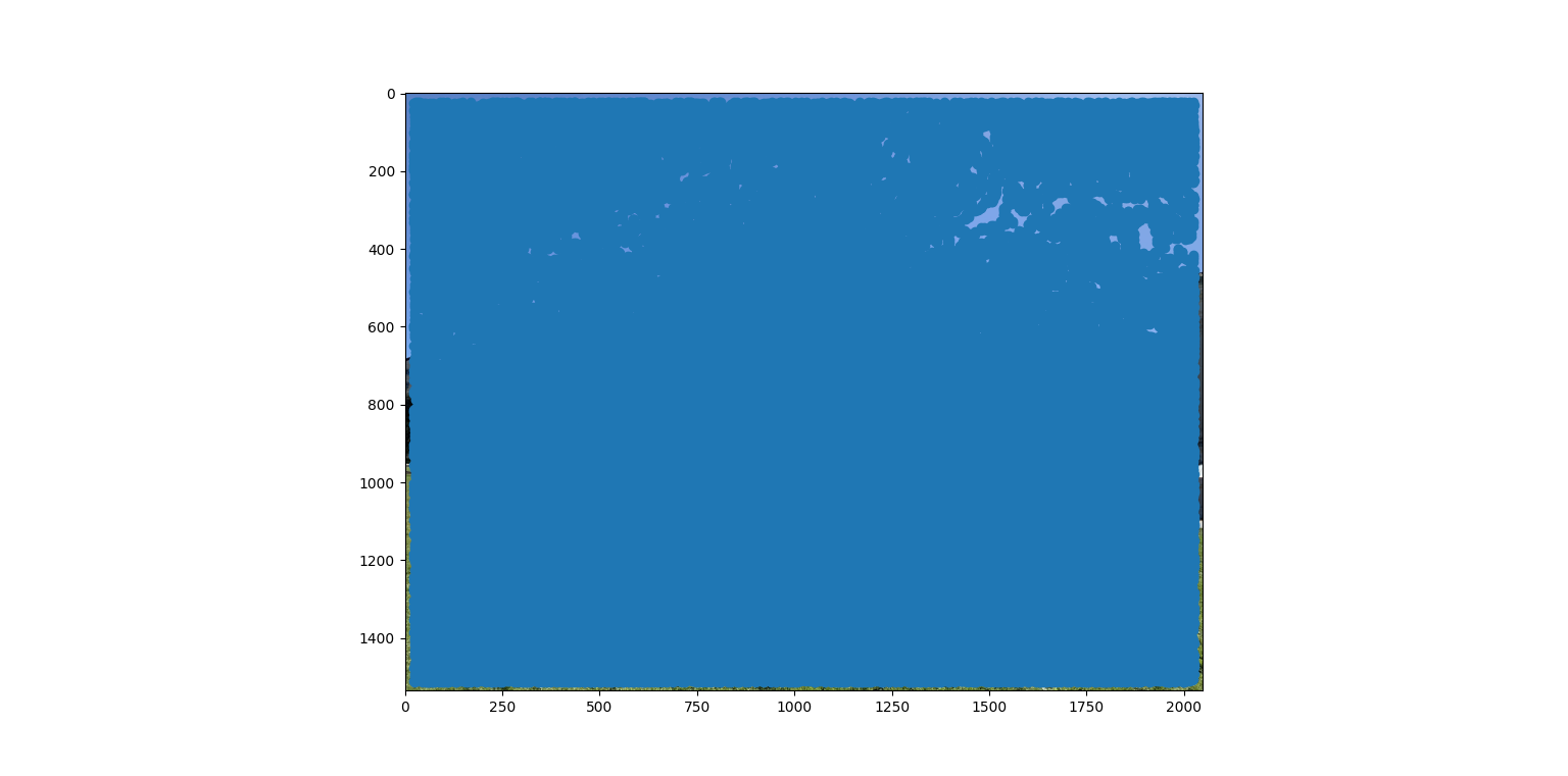
...oh.

So the Harris Corner Detector seems to think that everything is a corner. That's not super helpful. We need some way to suppress the points that aren't optimal ones for matching. Points that are the weakest "corners." Enter adaptive non-maximal suppression!!

ANMS

Adaptive non-maximal suppression allows us to get rid of all of the points that aren't the best in their localized area. Intuitively, ANMS selects out all of the local peaks in the image that are the best features for their neighborhood, and then matches our images based on those. This gives us a better estimate that uses fewer points and is thus both faster and more robust. After implementing ANMS, we get out an image that looks a little bit more manageable:

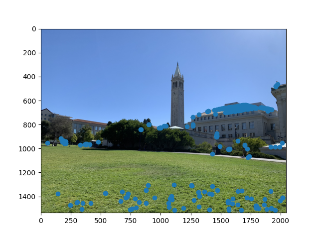
Notice that the points are a little bit more spread-out than before, and there are far fewer of them. This selection process will be extremely helpful in reducing the number of points as we move forward into the next part of our pipeline.

Feature Extraction and Matching

We used the grayscale intensity values of our images to match points, and the sum of squared differences to check if each set of points aligns with each other in the target image. We make sure to normalize these features before matching to make them invariant to slight intensity changes!

RANSAC Matching

The final part of our algorithm is to compute our homography and transform our image. This can easily be done by using the Random Sample Consensus (RANSAC) algorithm, using our matched points from the previous parts. By randomly drawing from our points and taking the best homography out of each random combination, this algorithm allows us to find the best options in far less time than exhaustive search. We are able to compute a near-perfect homography between our two images, no-human required, in relatively quick fashion. And here are some of the results!

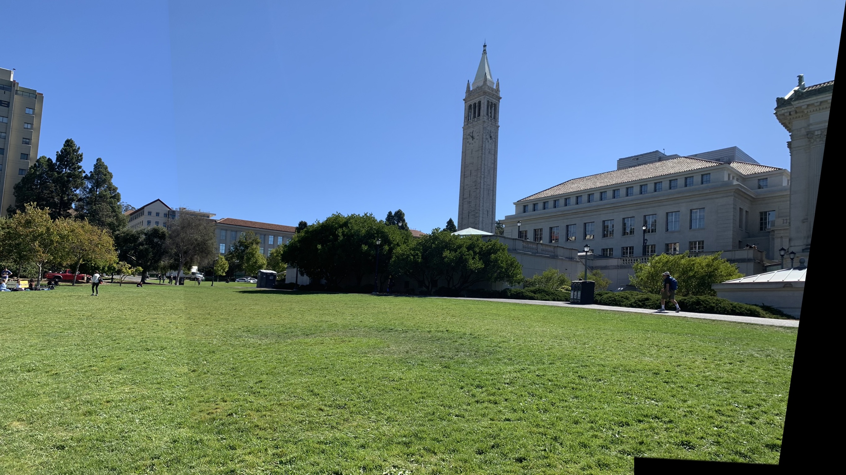
(I messed up and forgot to lock the exposure on this one, thus the slight color change between the two halves of the photo, but it still matches the positions well)