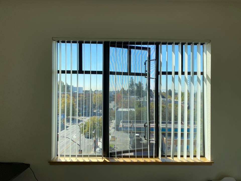
Part.1 Shoot the pictures
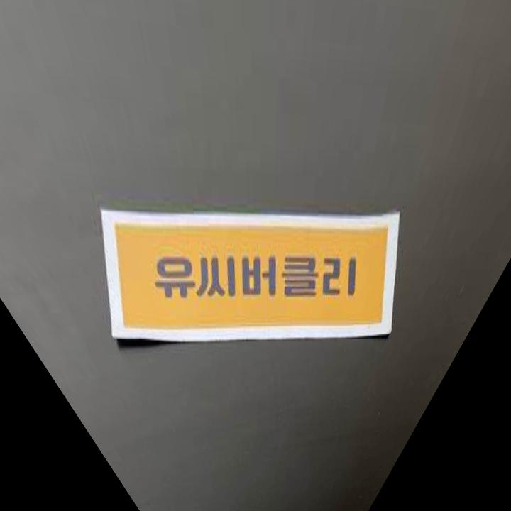
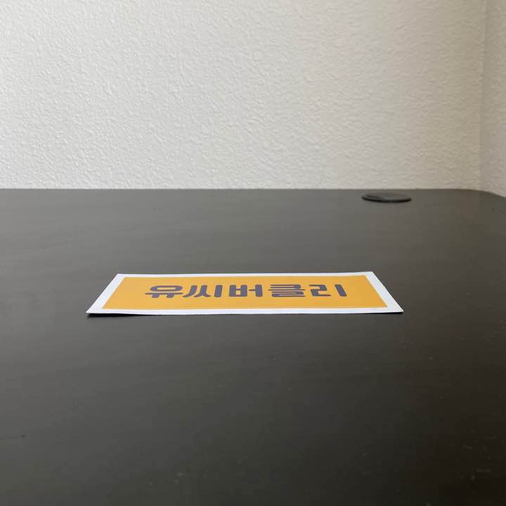 sticker sticker
|
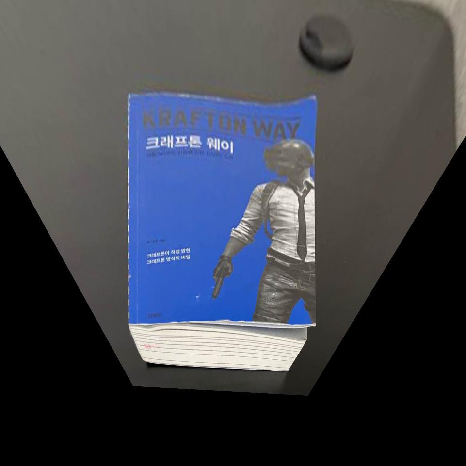
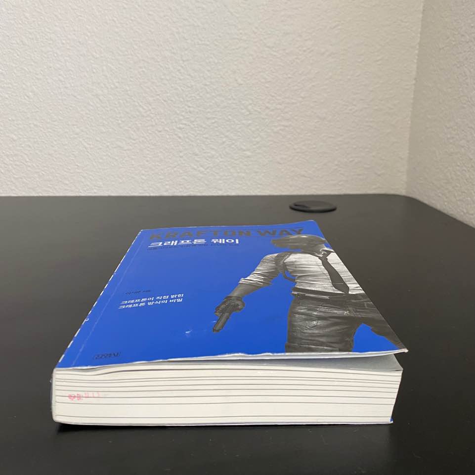 book book
|
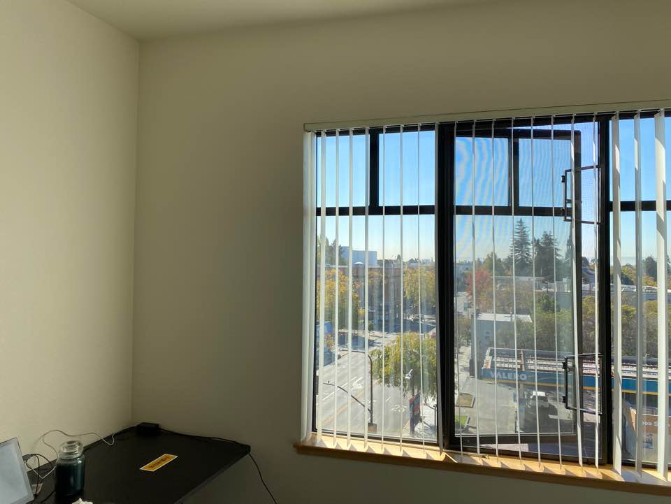
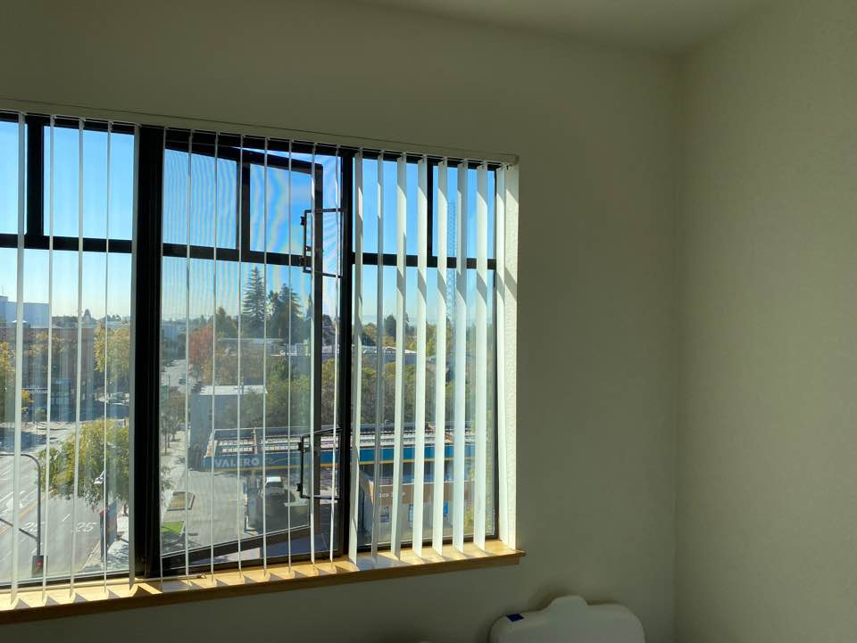
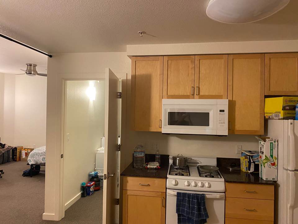
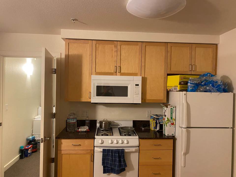
The images above are going to be used as an example to simply show the change of viewing angle.
The images above are going to be used as an example to show the change of viewing angle. And then, the images would be used to be stitched to create a panoramic image with mosaicing.
Part. 2 Recover Homographies
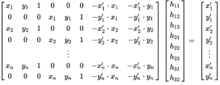
Homography refers to the matrix that allows the projective transformation from one image to the other image. And for use, this is used to change the viewing angle. Solving the following matrix for h vector will give us the necessary points for homographies.
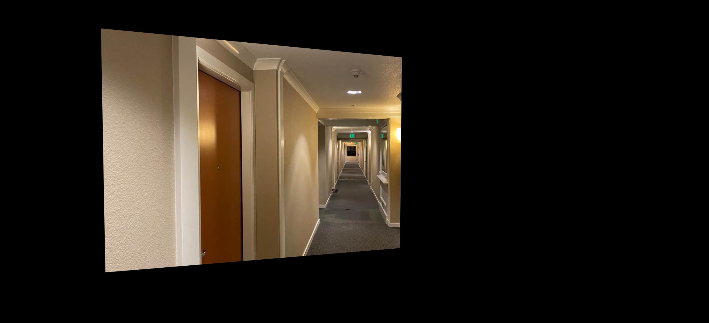
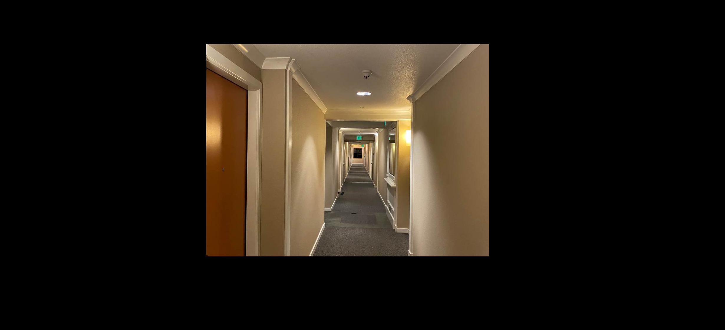
Part. 3 Warp the Images
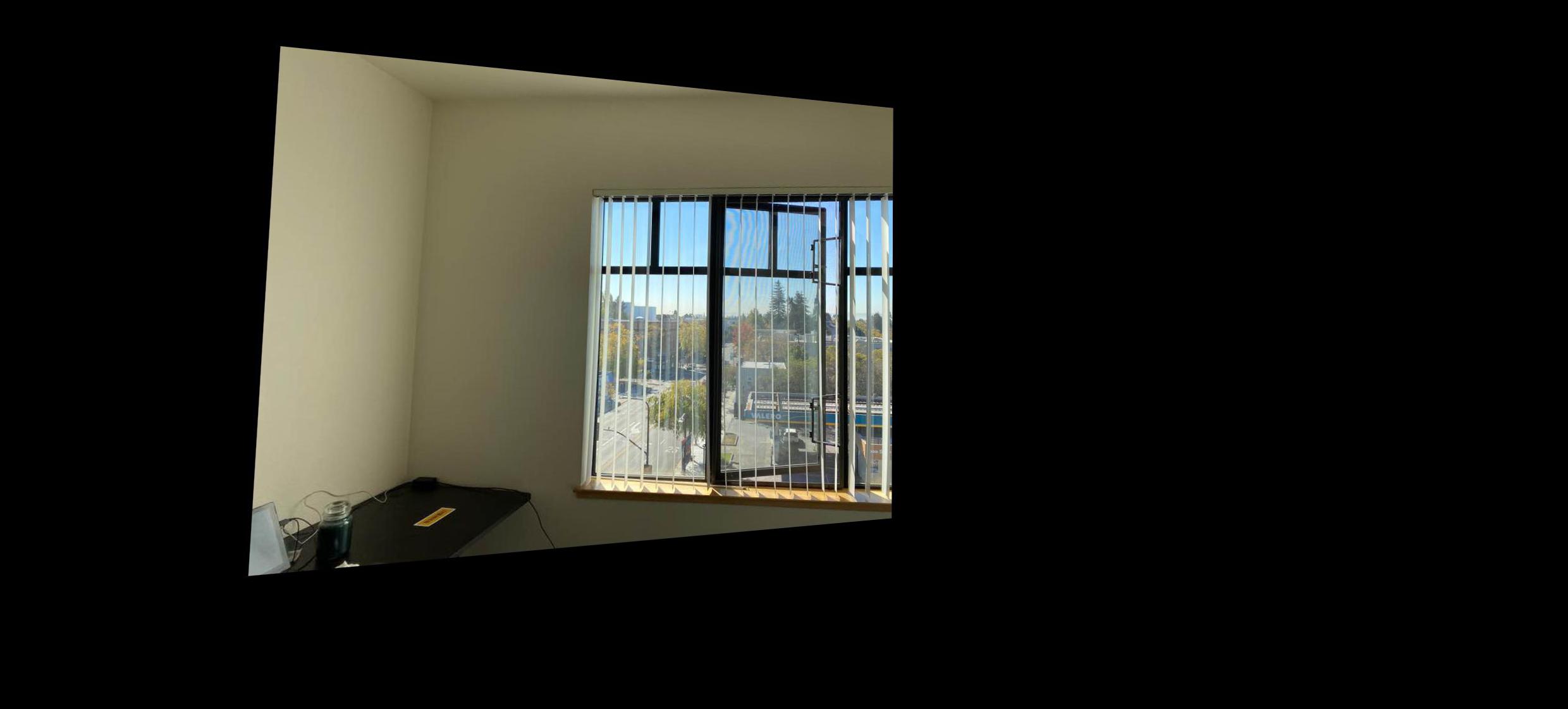
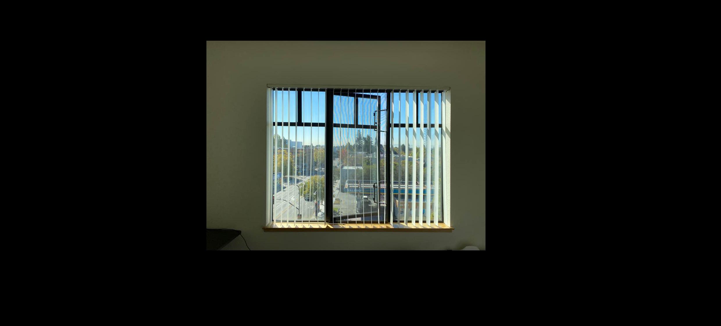
As we obtained the homographies, now we can apply inverse warping to get the image of changed viewing angle. And the following images are some of those examples. I tried to show how the object in front would look like if we changed the viewing angle as we are looking from top to bottom.
|
sticker
|
 rectified rectified
|
|
book
|
 rectified rectified
|
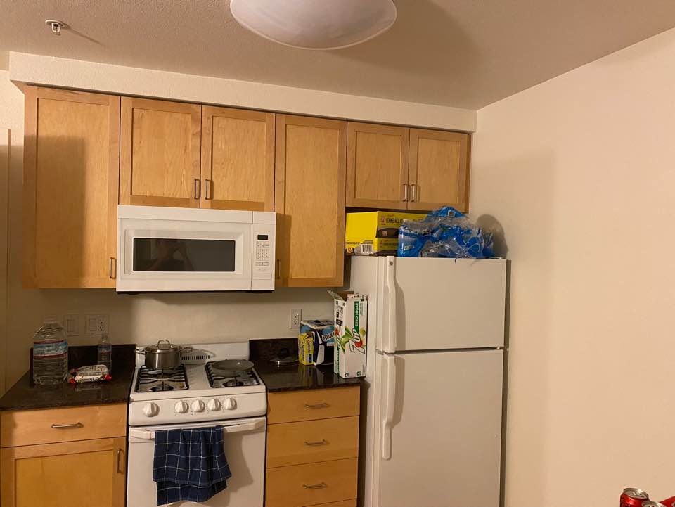
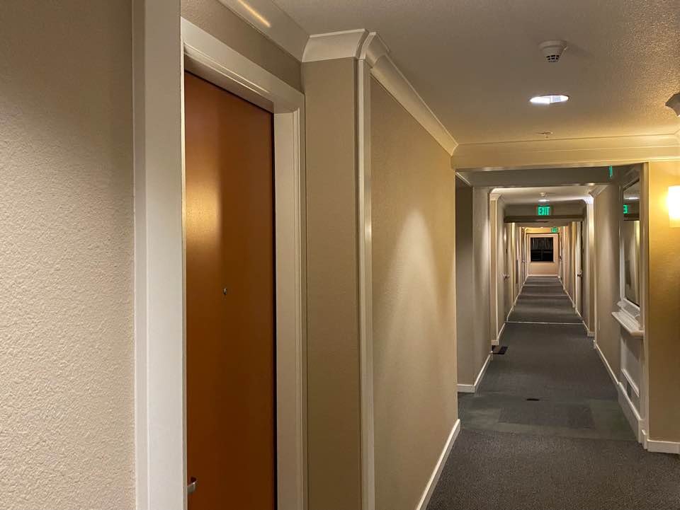
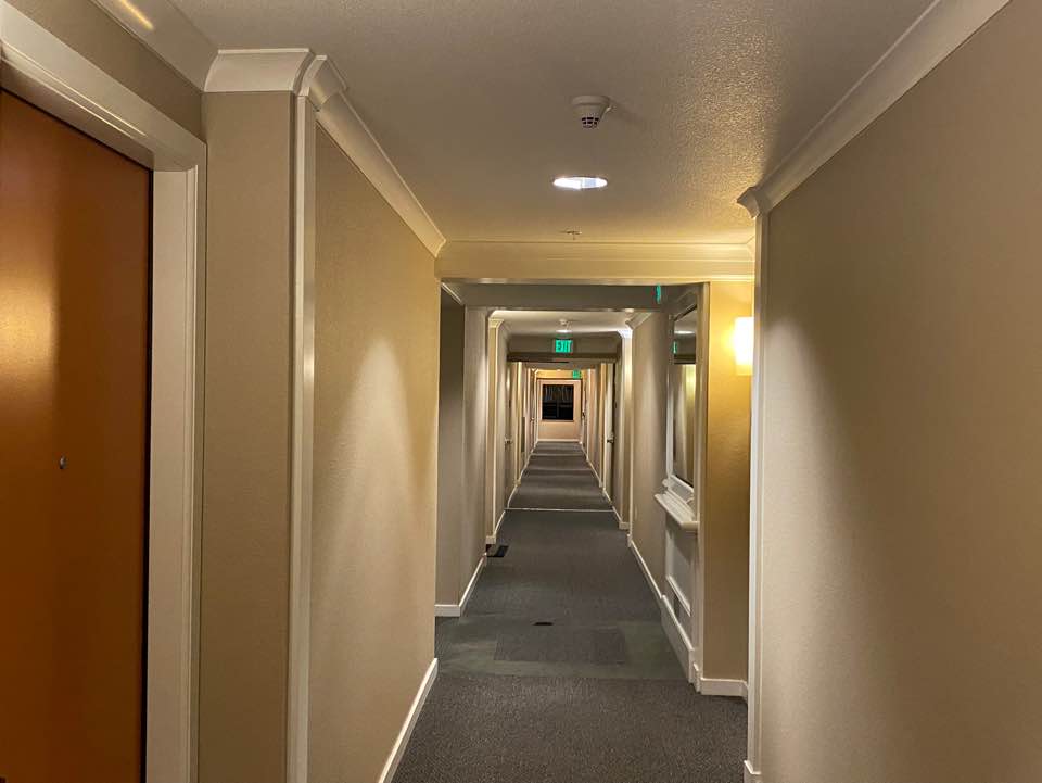
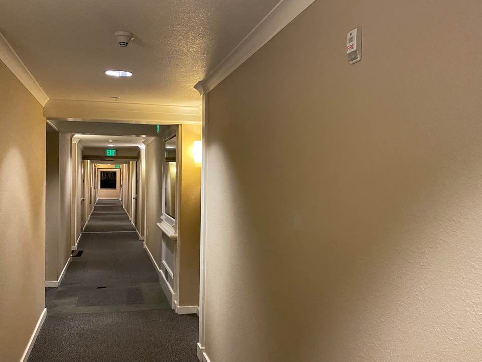
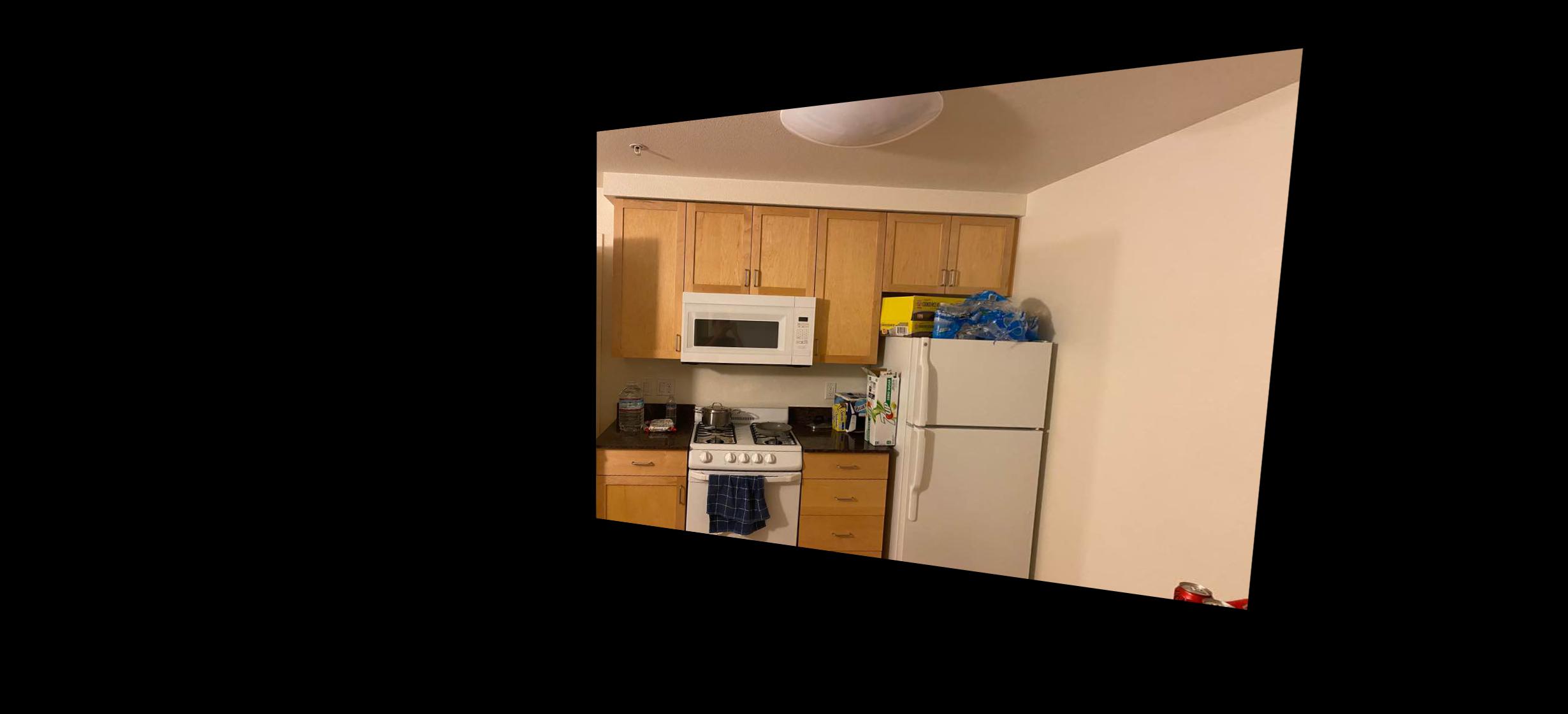
Part. 4 Blend Images into a Mosaic
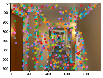
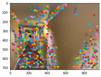
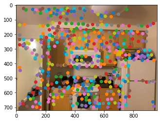
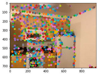
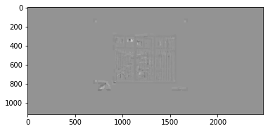
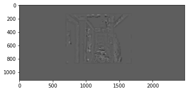
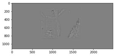
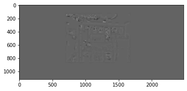
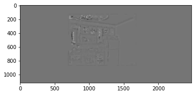
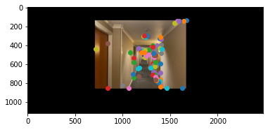
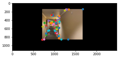
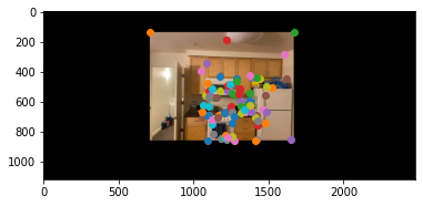
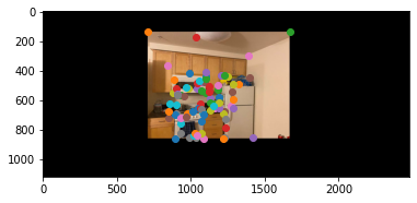
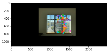
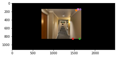
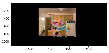
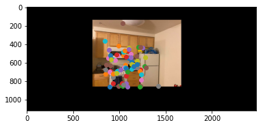
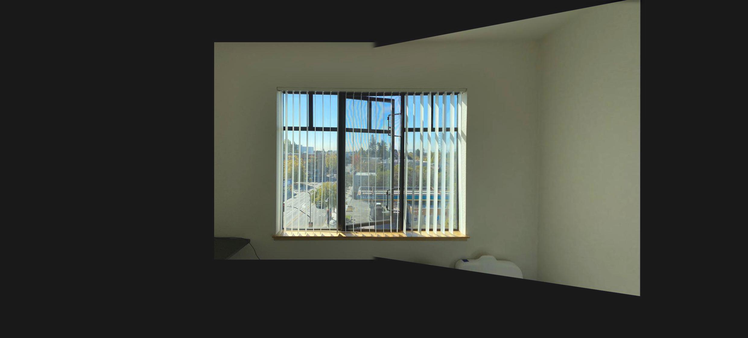
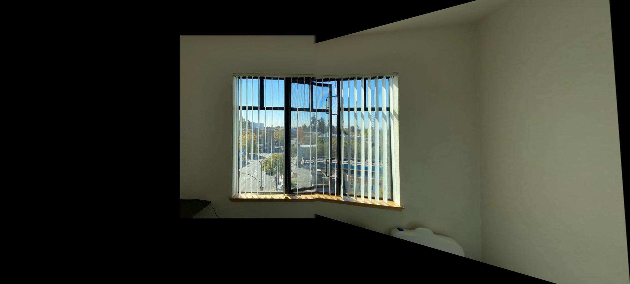
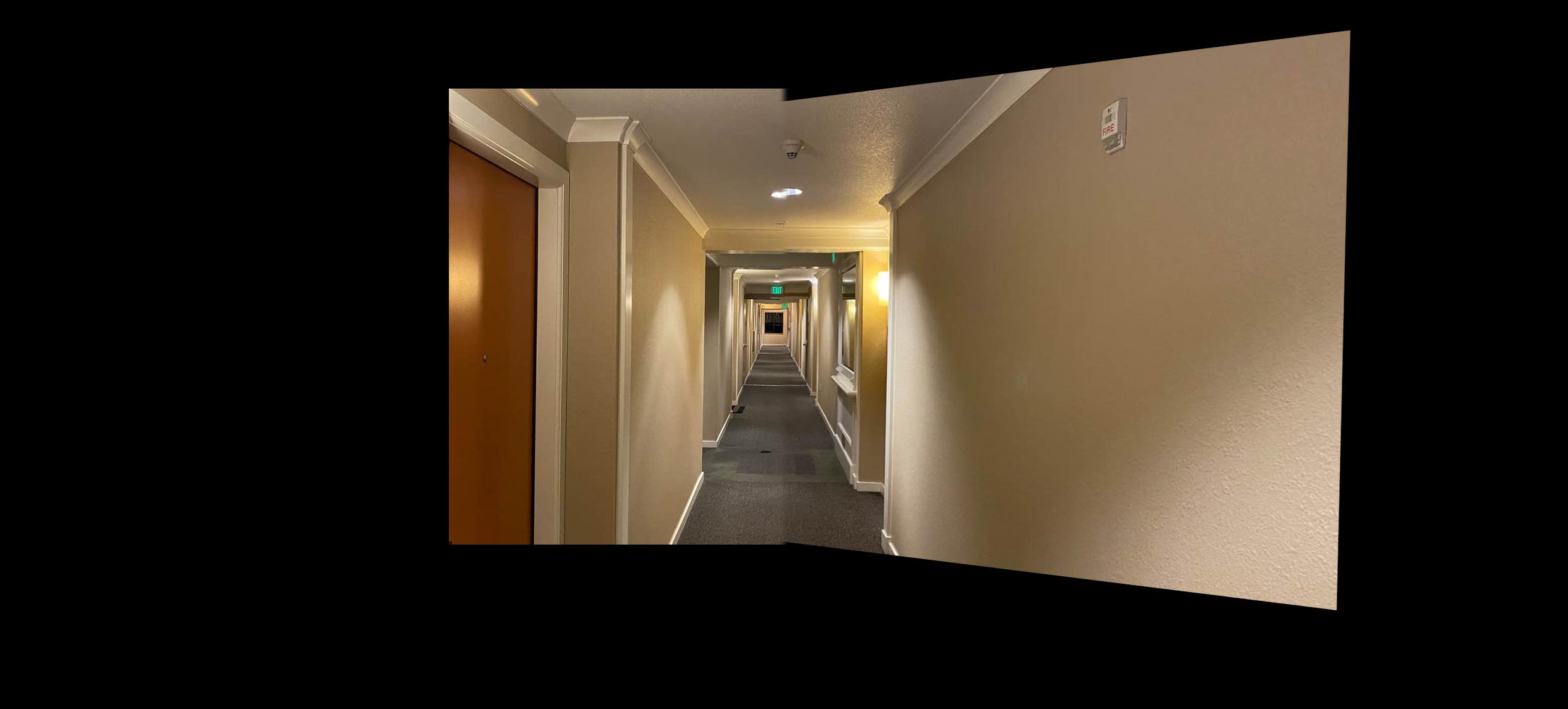
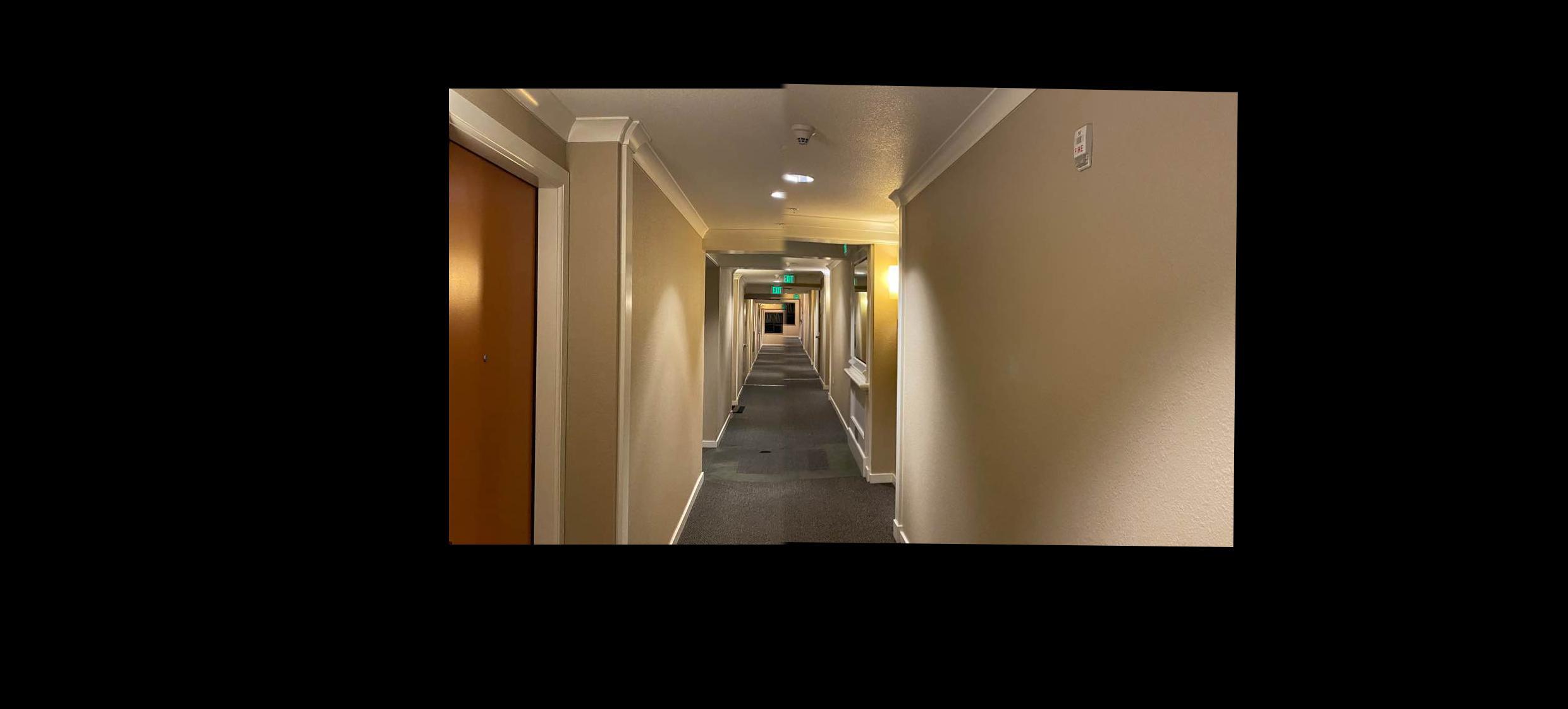
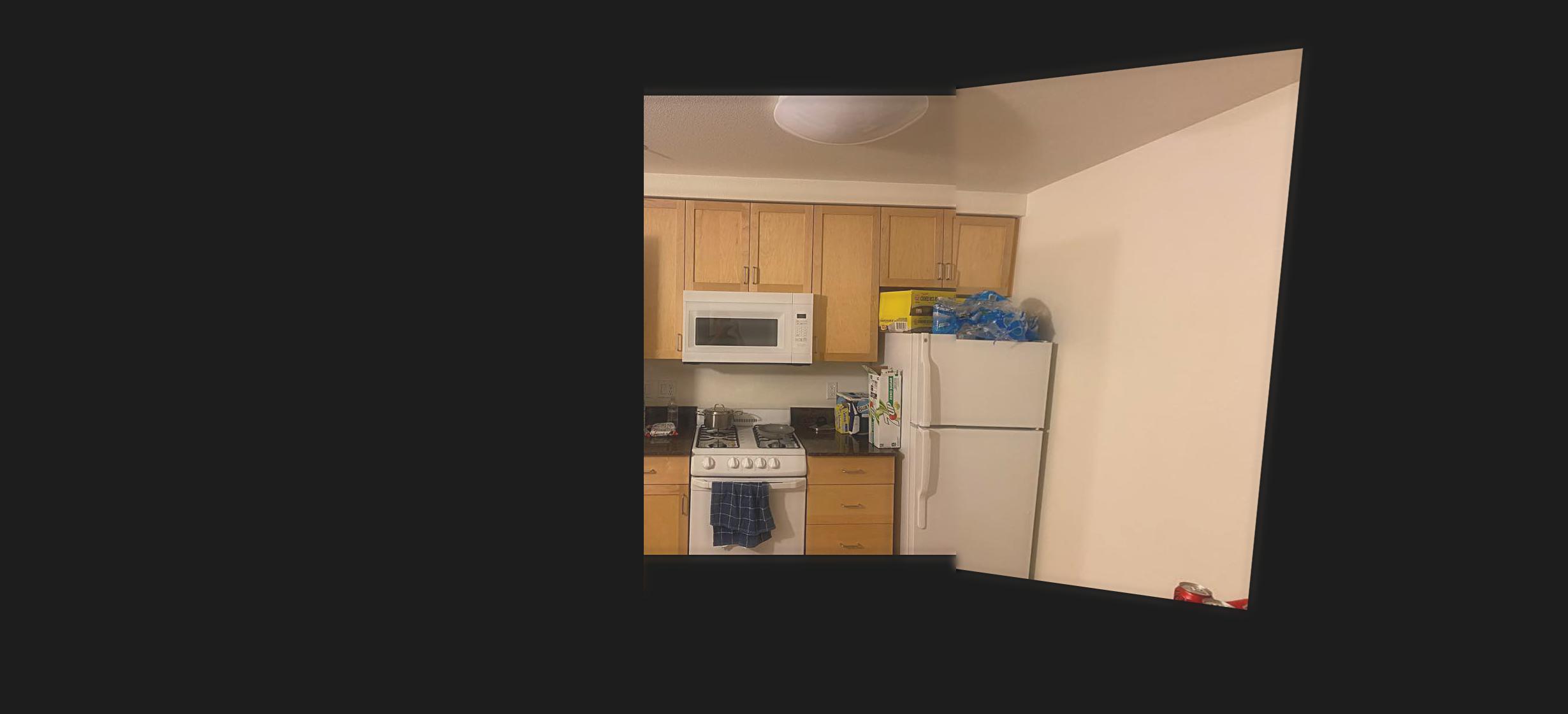
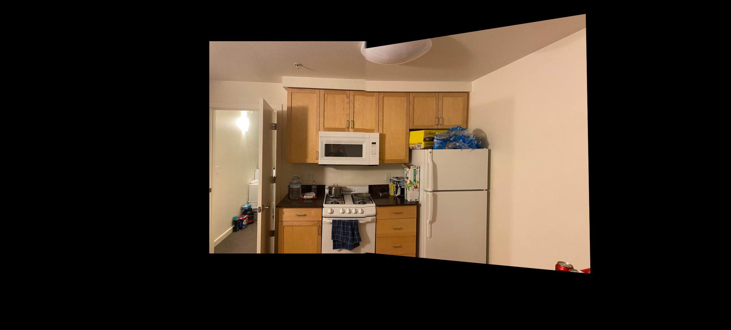
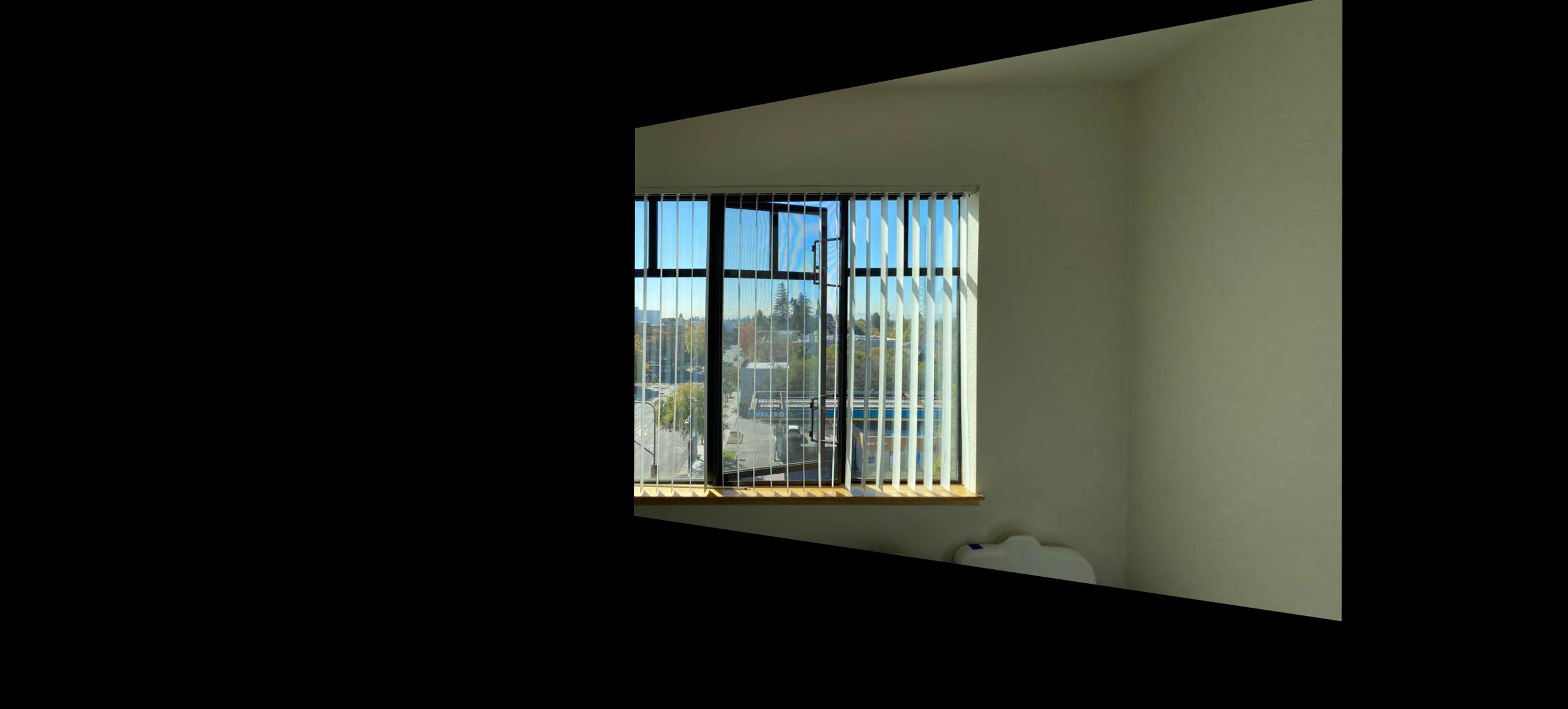
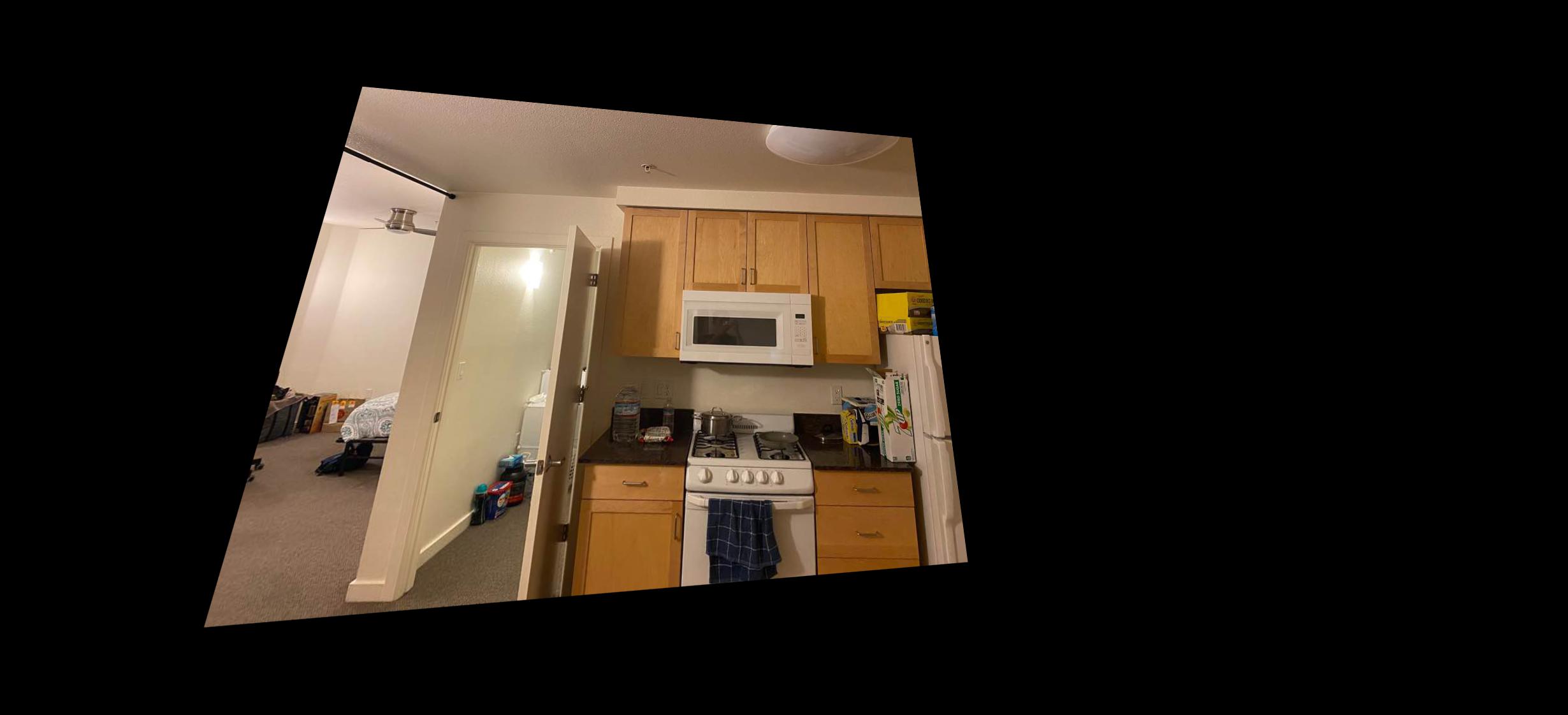
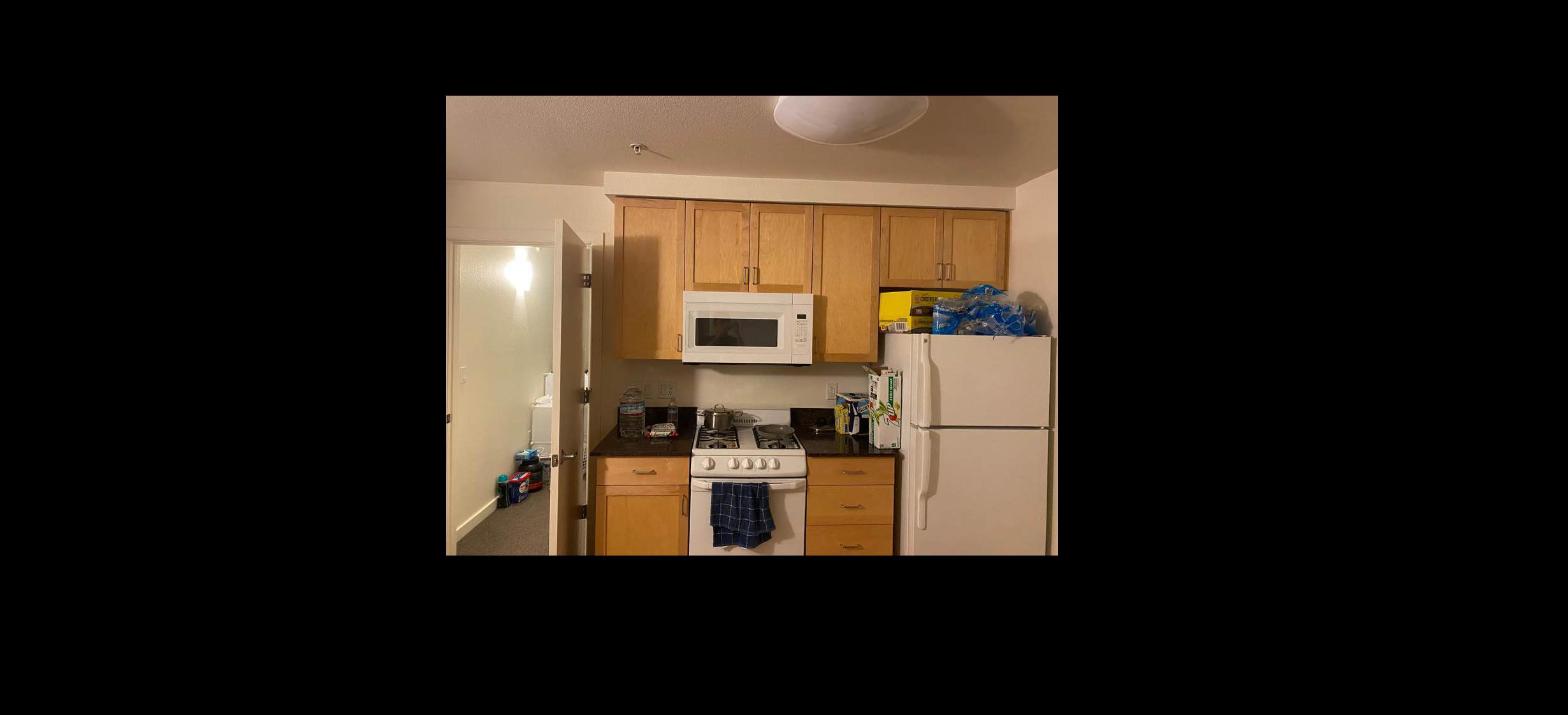
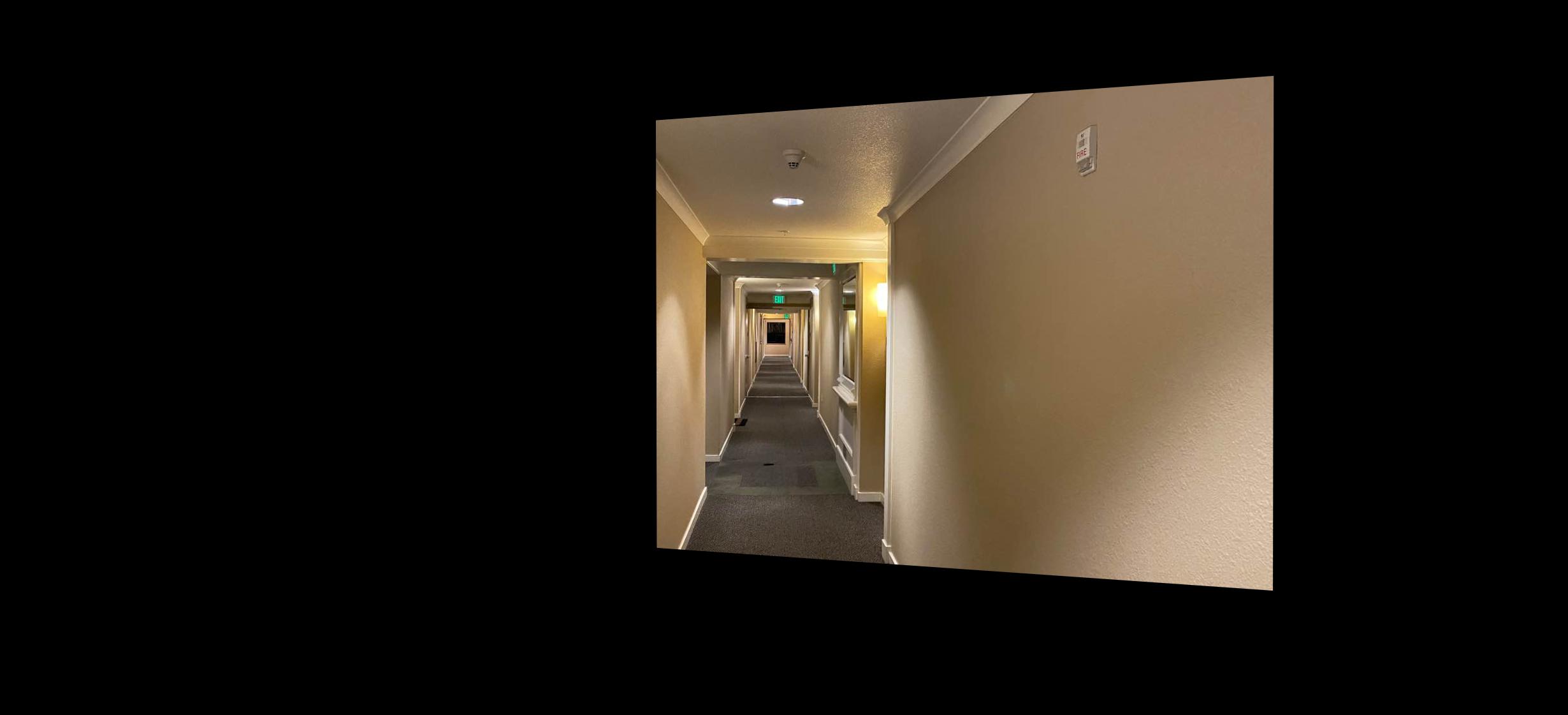
Using the same idea from part 3, I can rectify images and stitch them together to create a panoramic image. We first pad the images so we do not lose information. Then, obtain the common points between the images in order to stitch them in a correct way.
 rectified rectified
left
|
 rectified rectified
middle
|
 rectified rectified
right
|
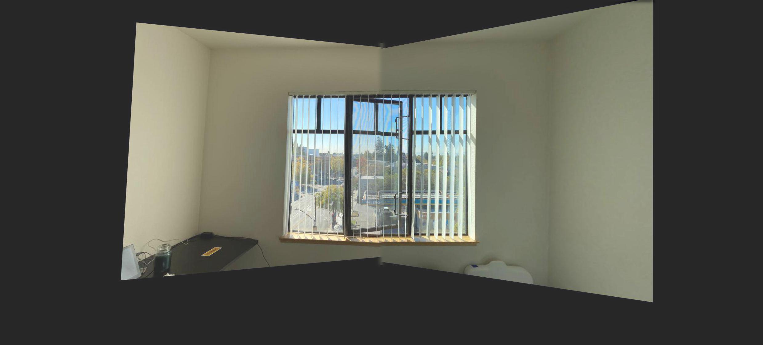 blended blended
|
 rectified rectified
left
|
 rectified rectified
middle
|
 rectified rectified
right
|
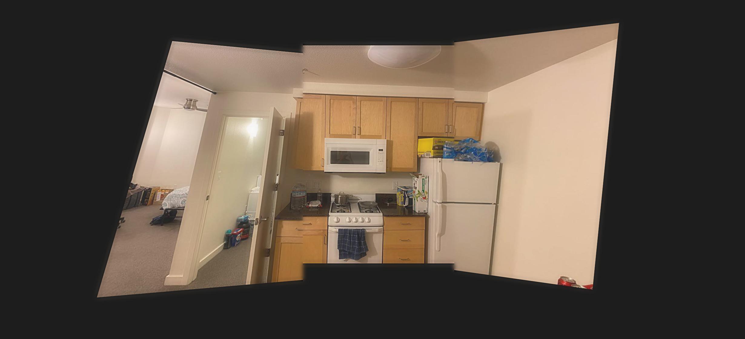 blended blended
|
 rectified rectified
left
|
 rectified rectified
middle
|
 rectified rectified
right
|
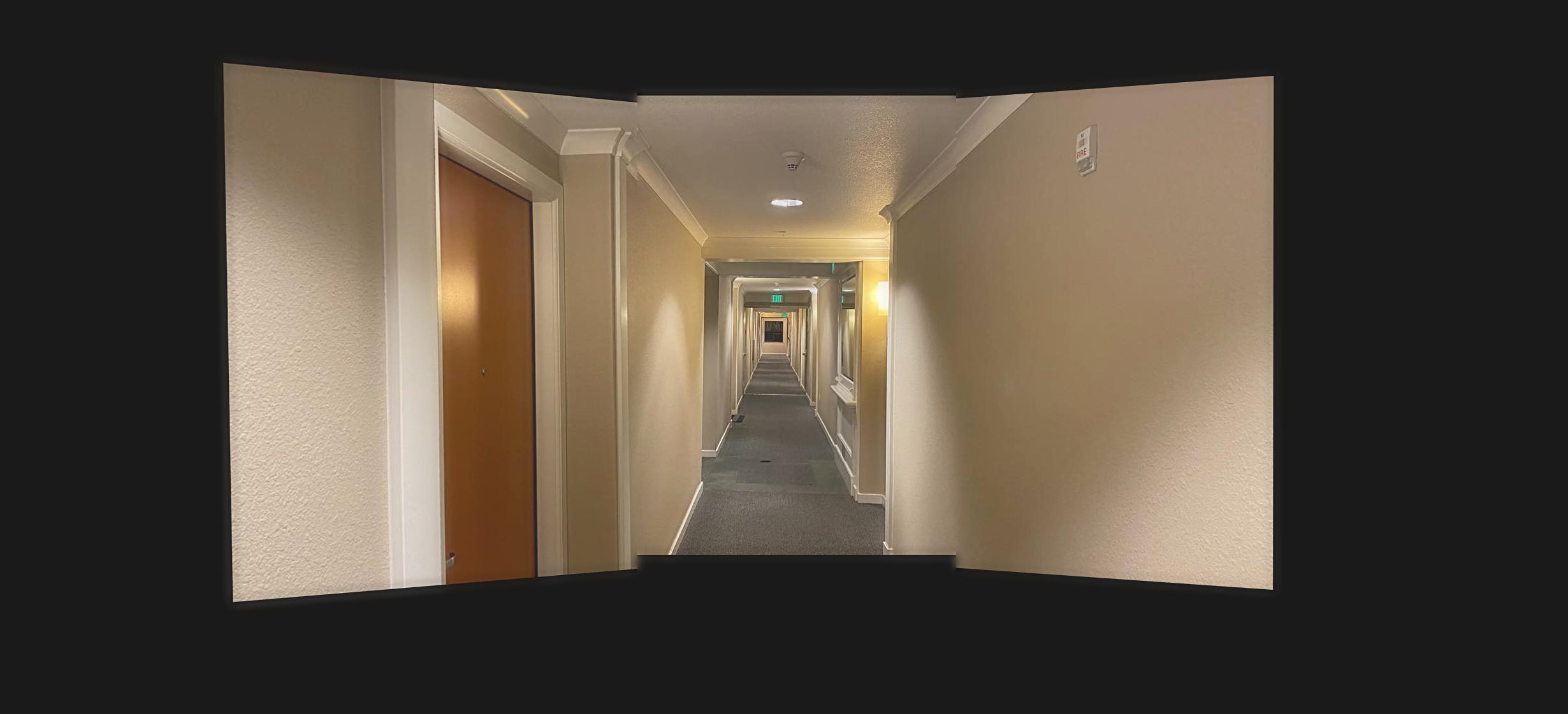 blended blended
|
Project 4B Overview
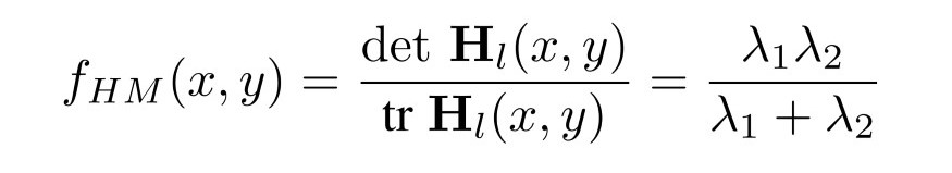
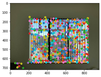
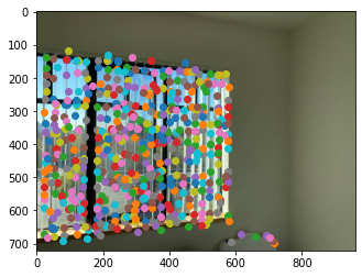
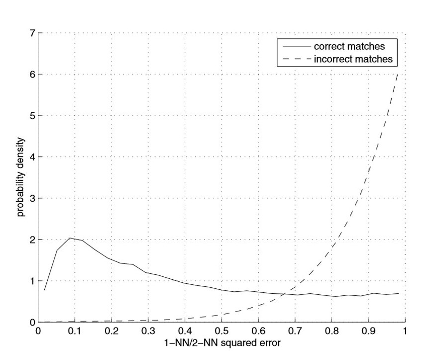
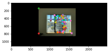
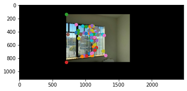
Opposed to manually selecting the points to compute the homography from project 4A, now we discover a way to select points automatically using harris corners, feature descriptors, feature matching, and RANSAC. This way, we can automatically stitch images without any manual work.