Part 1: Shoot the Pictures
The goal of this part is to take pictures that can be aligned and blended into a mosaic. It was important to take pictures standing from the same location, just rotating the persepctive of the camera. The pictures should also have a significant amount of overlap, allowing us to select correspondence points between images for alignment purposes. I also took pictures of items that would be used for image rectification. I made sure that these items were rectangular in nature, but due to camera perspective, they would appear slanted in the original image.
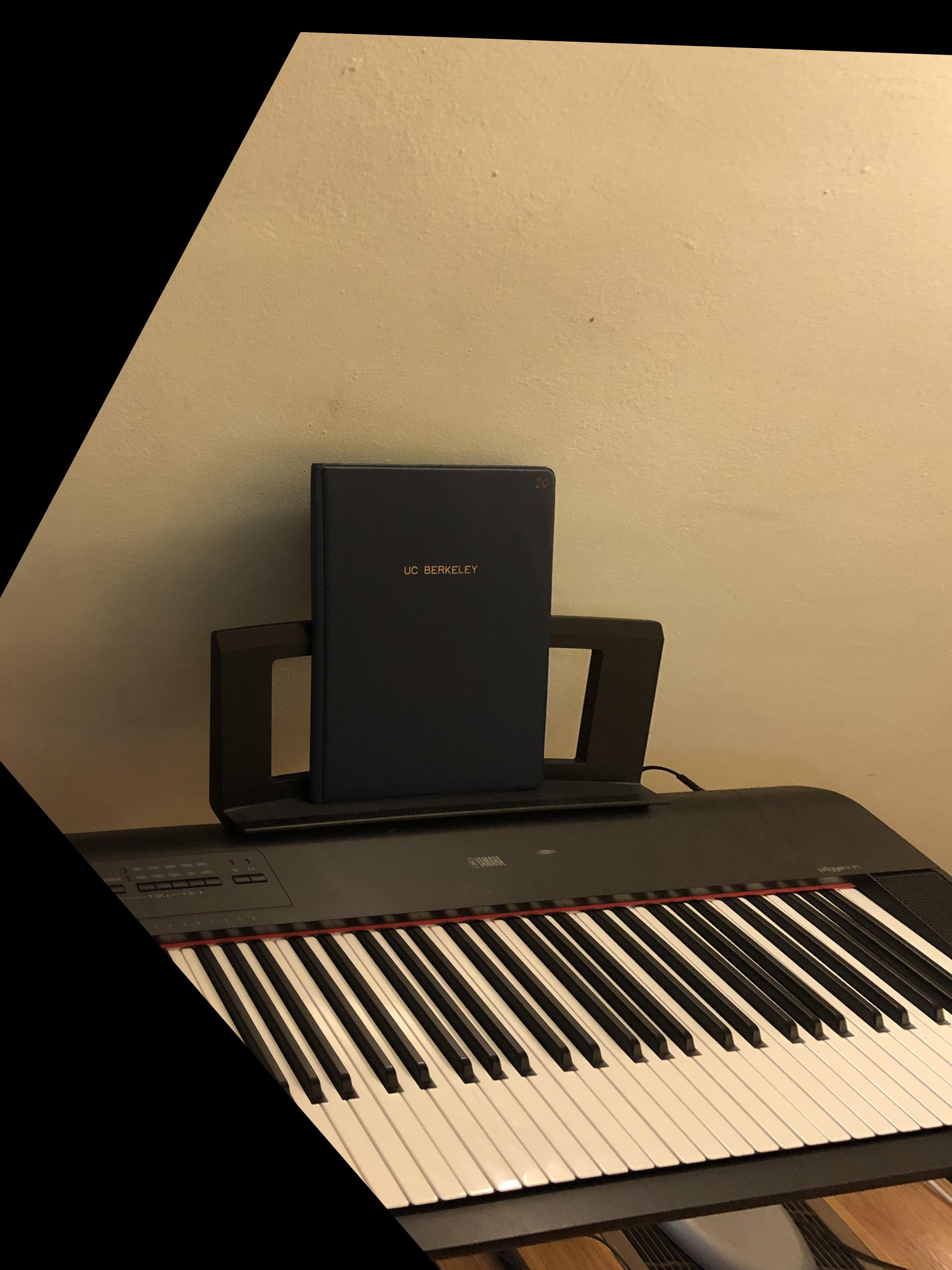
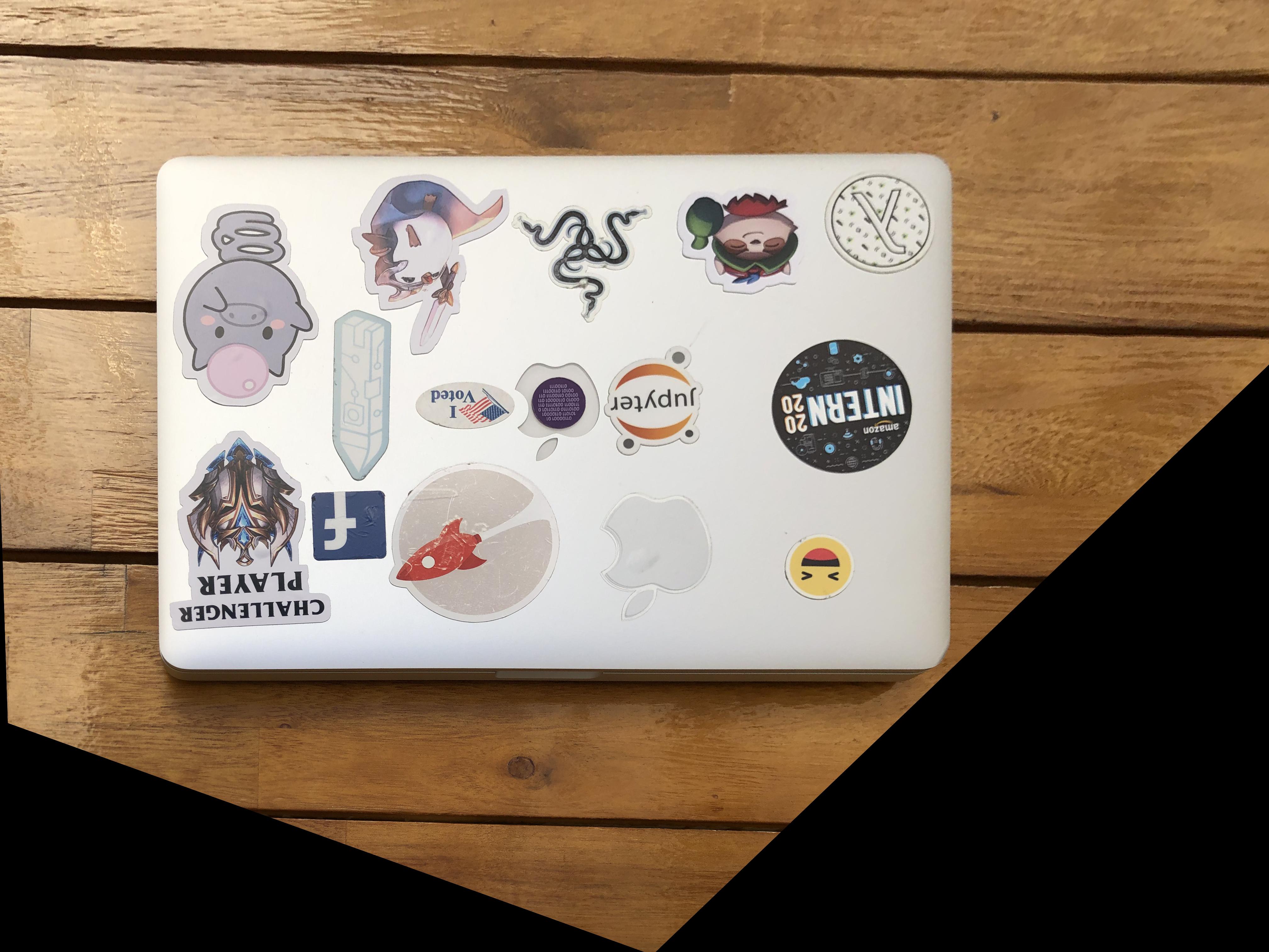
Images for rectification:
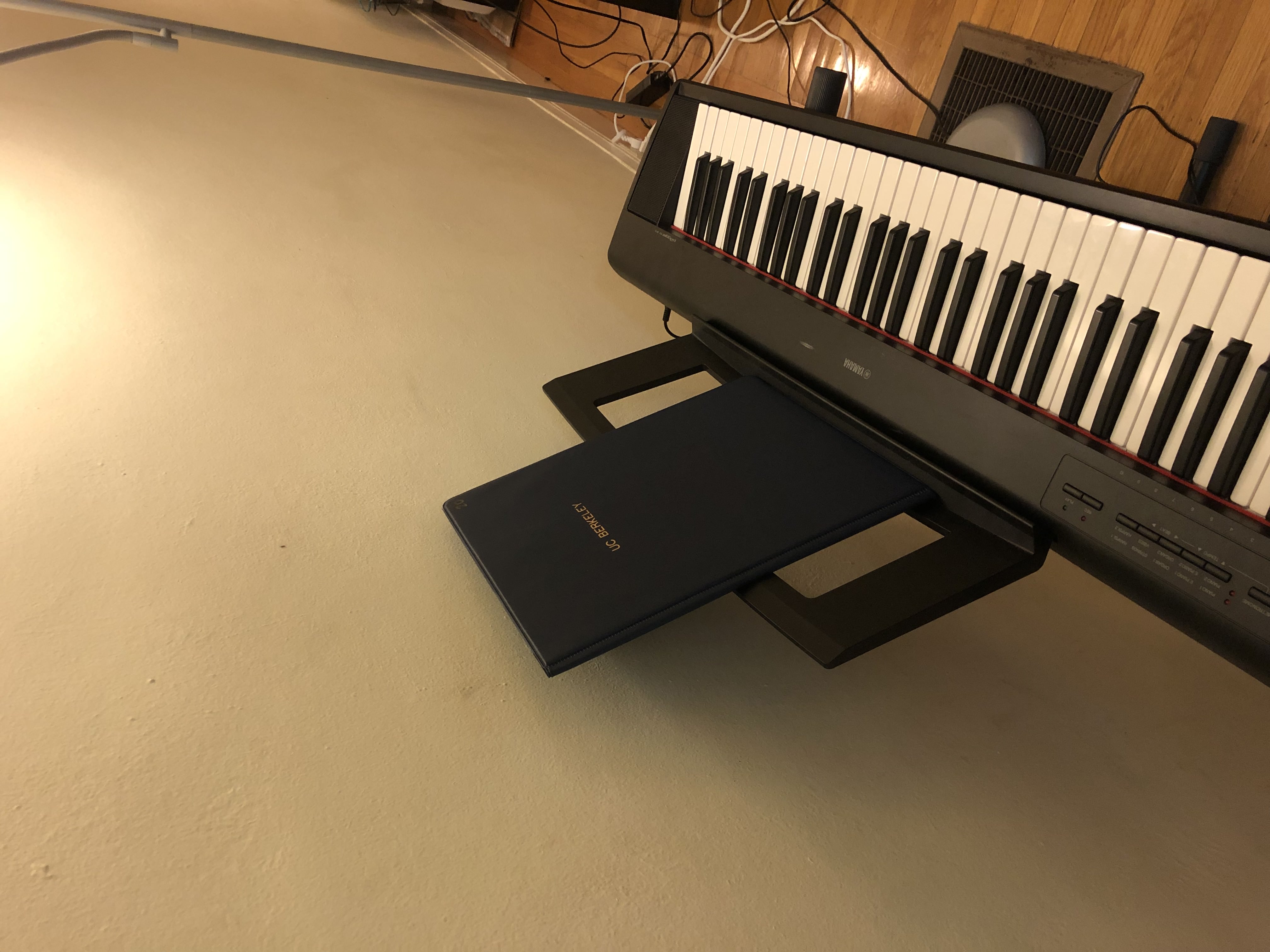
Music Folder
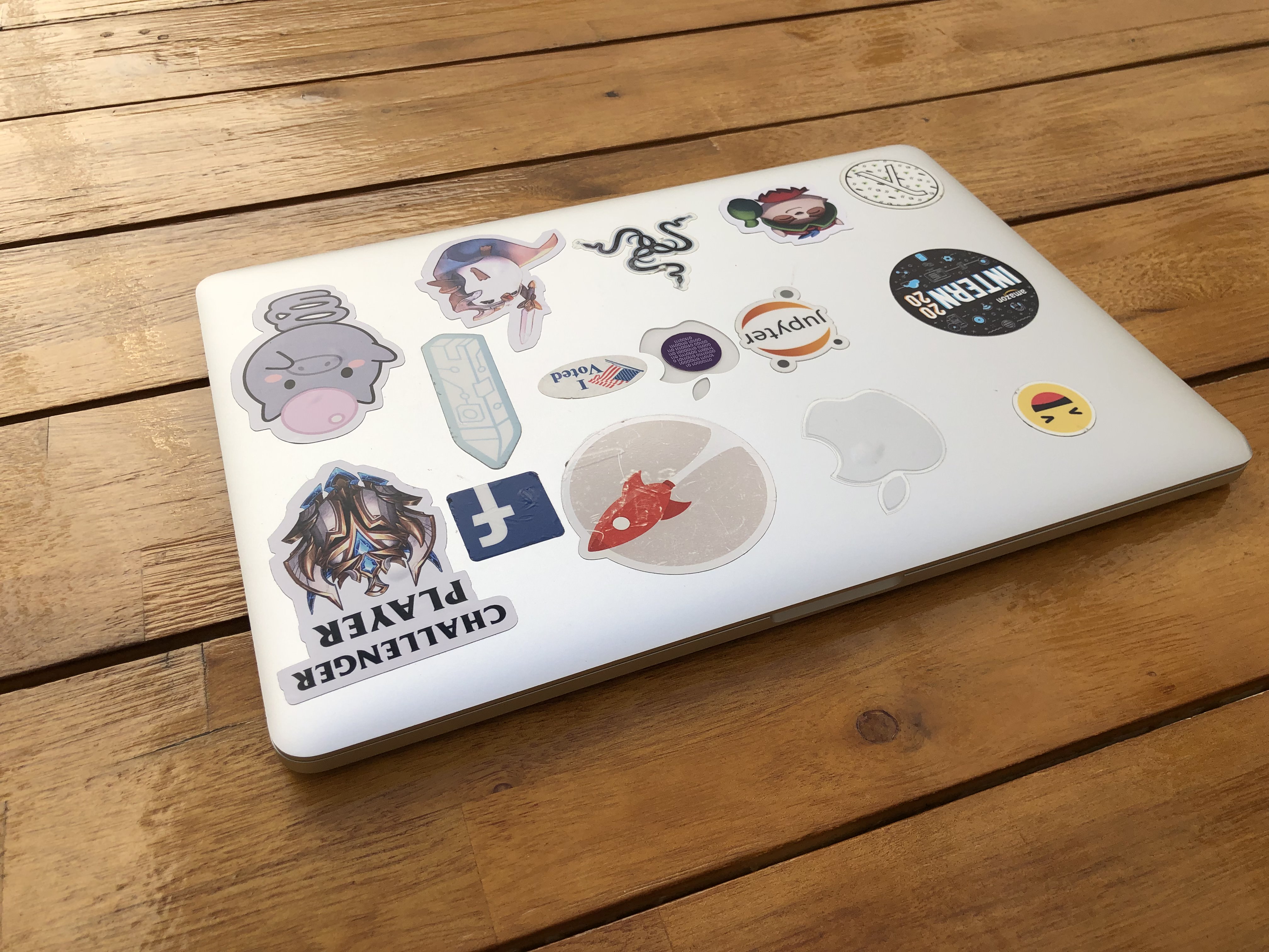
Laptop
Mosaic Image Sets
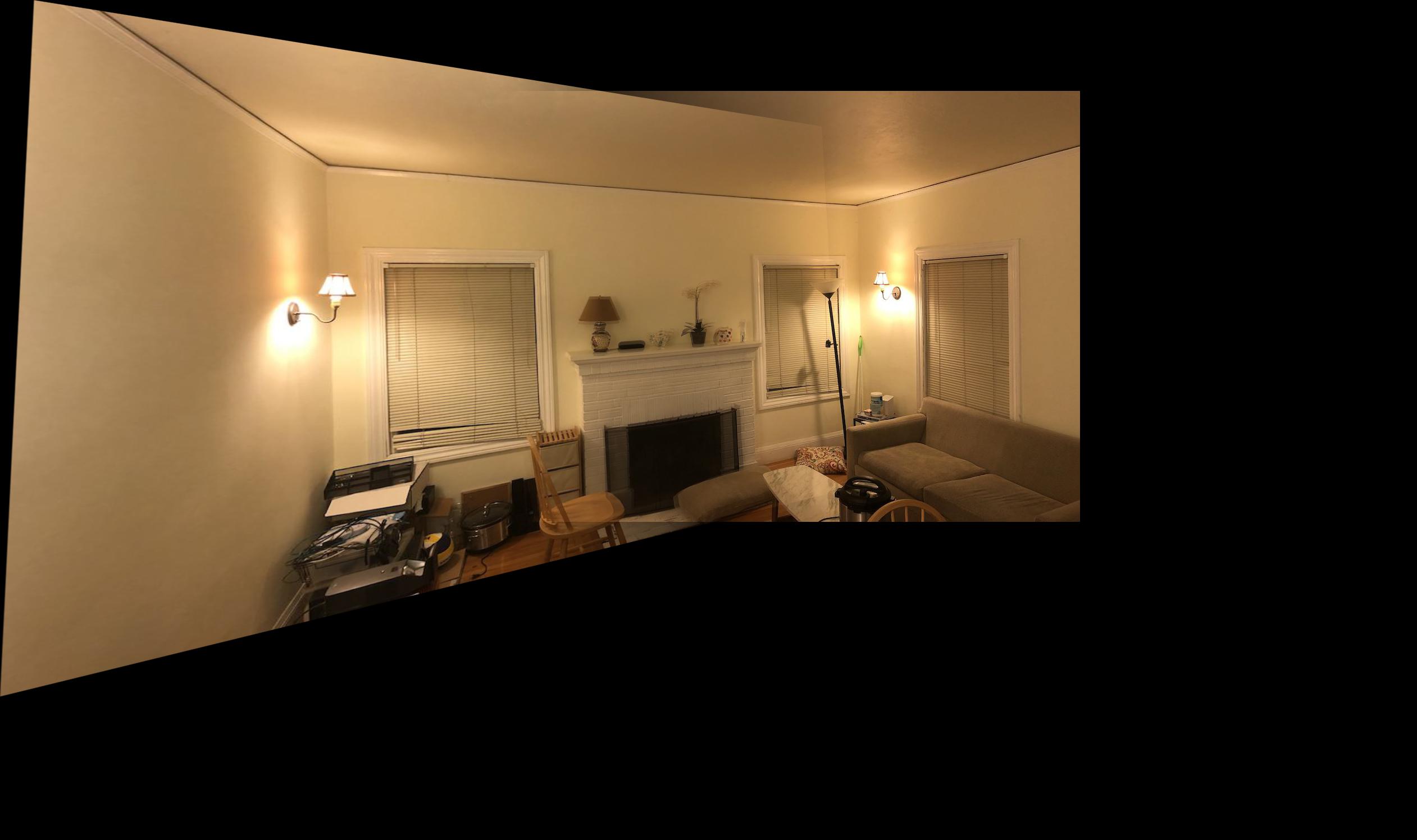
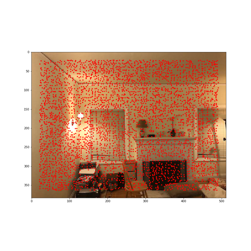
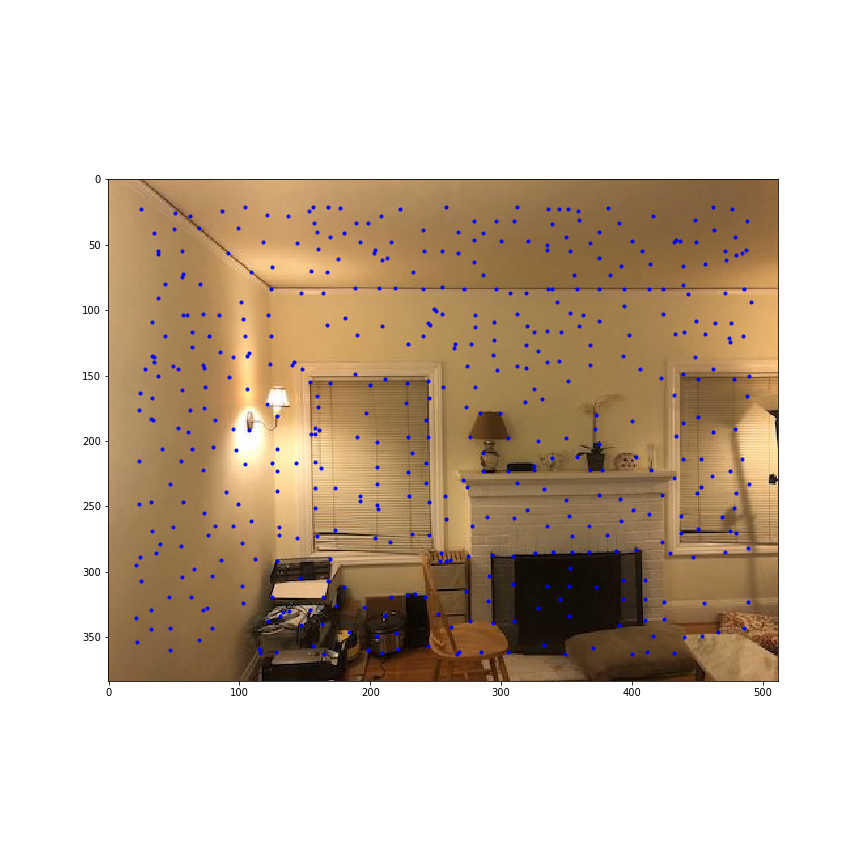
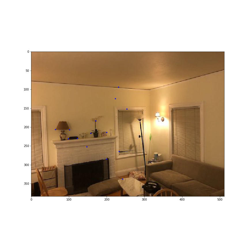
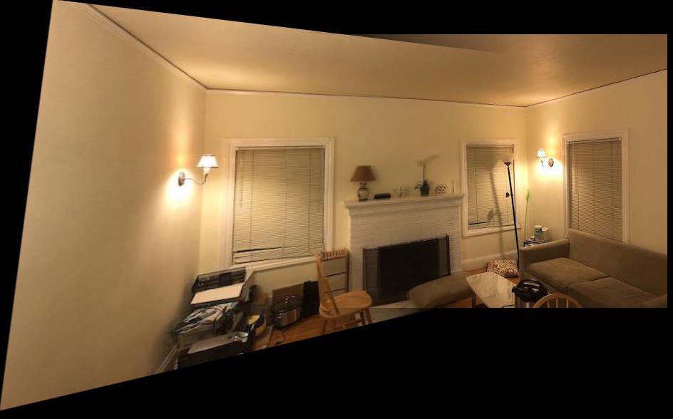
Image Set 1: Living Room
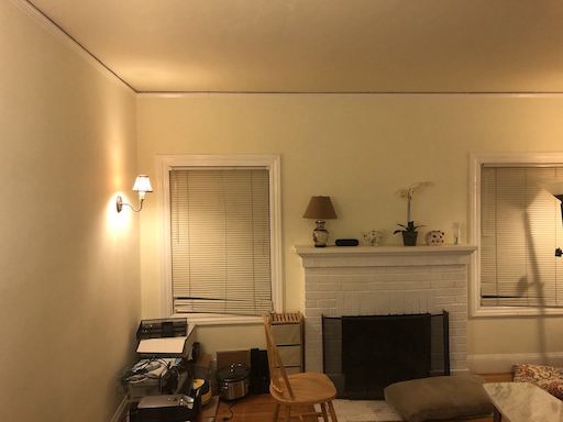
Living Room Left
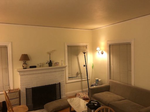
Living Room Right
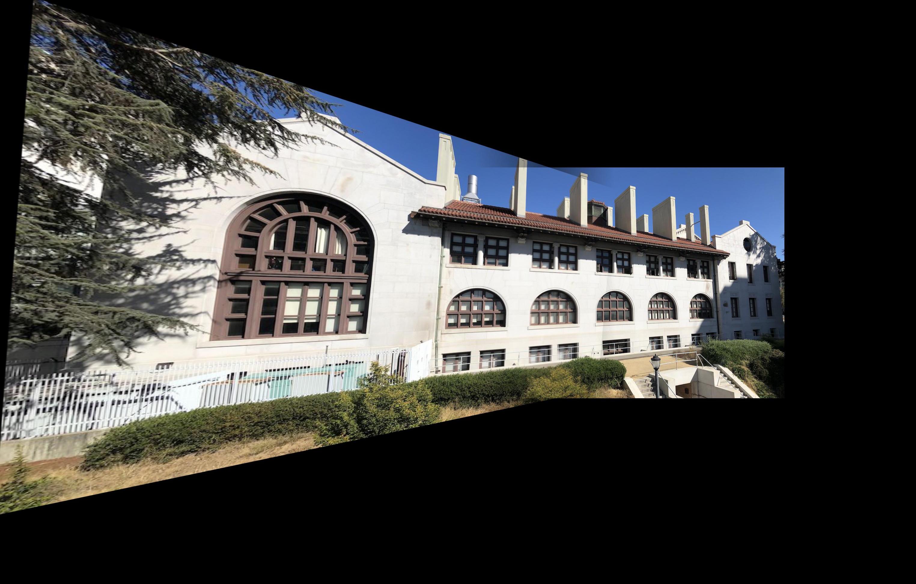
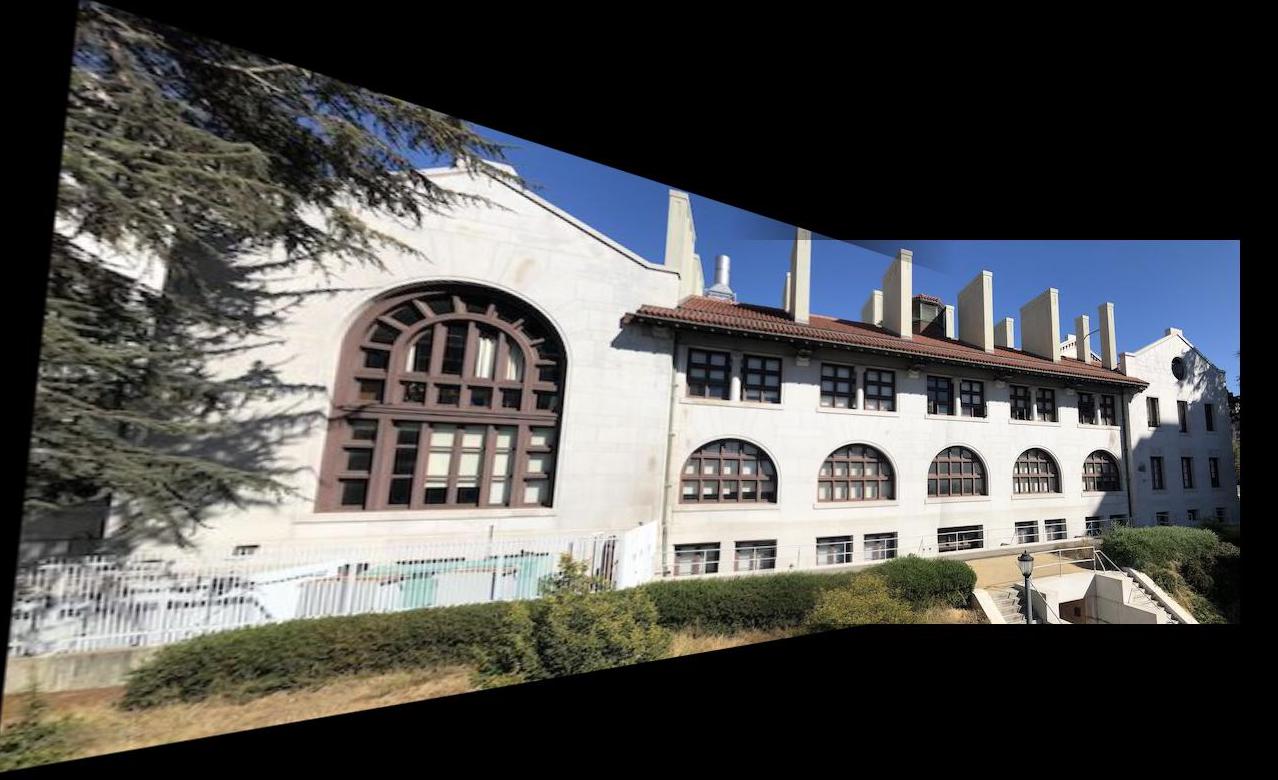
Image Set 2: Side of HMMB
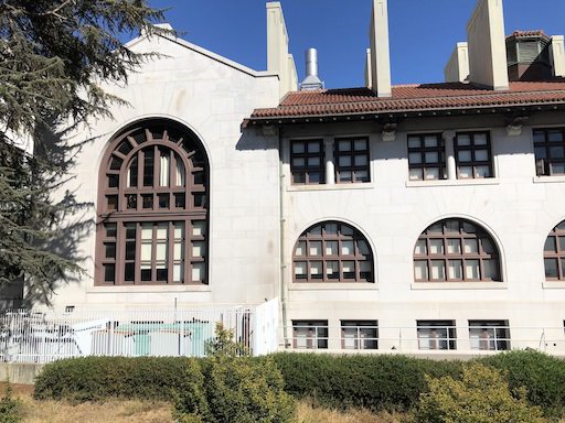
HMMB Left
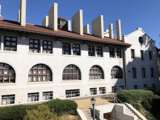
HMMB Right
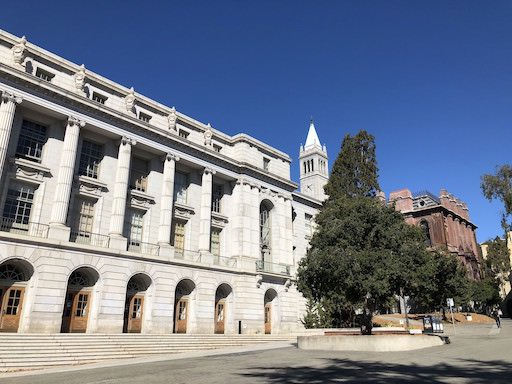
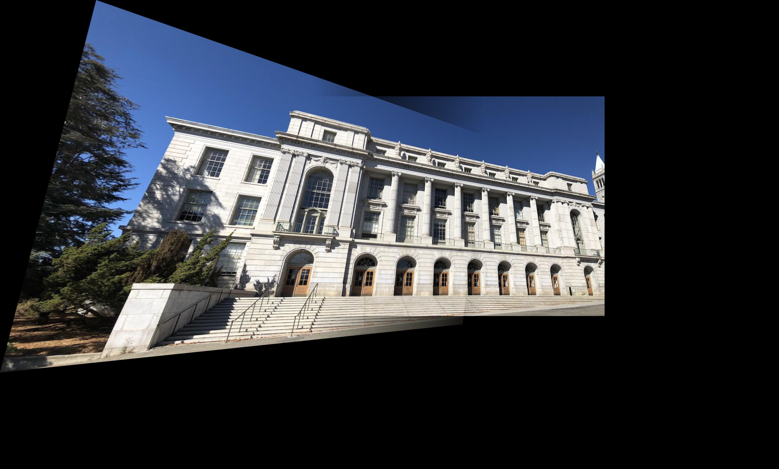
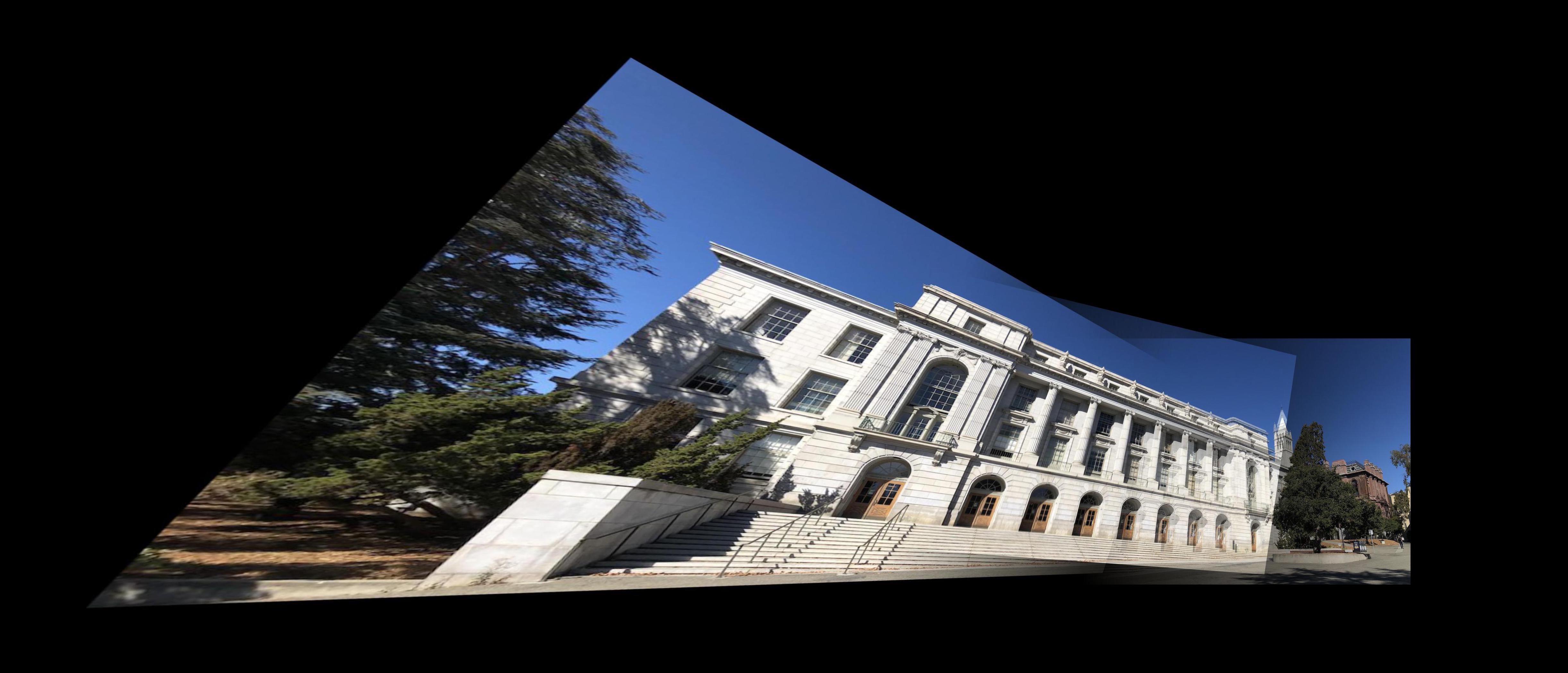
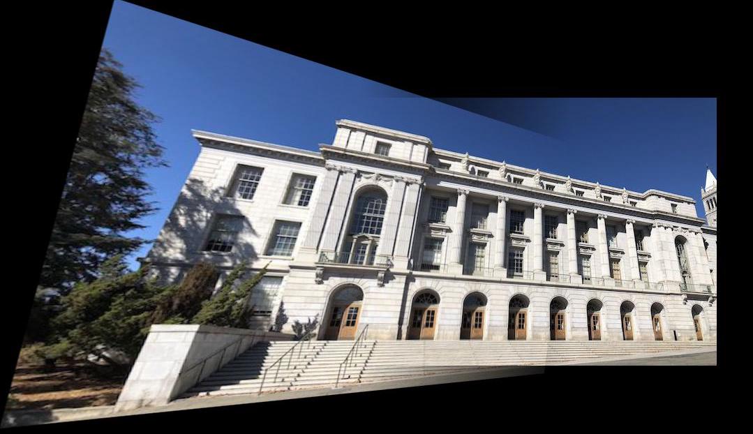
Image Set 3: Wheeler Hall
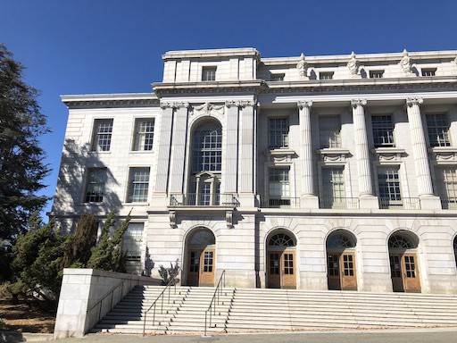
Wheeler Hall Left
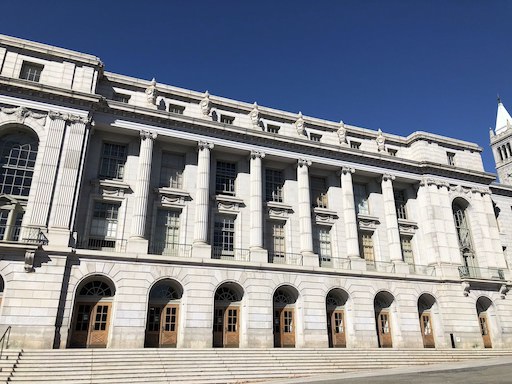
Wheeler Hall Middle