Part A
Shoot the Pictures
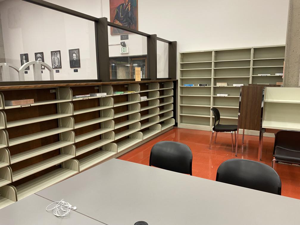
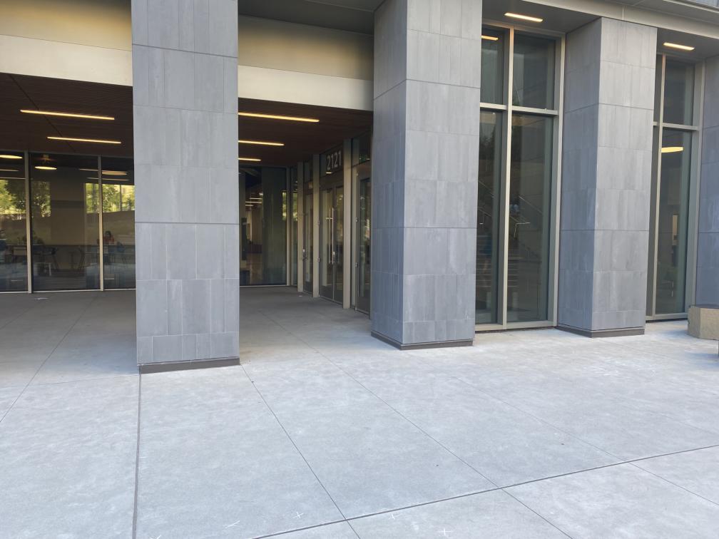
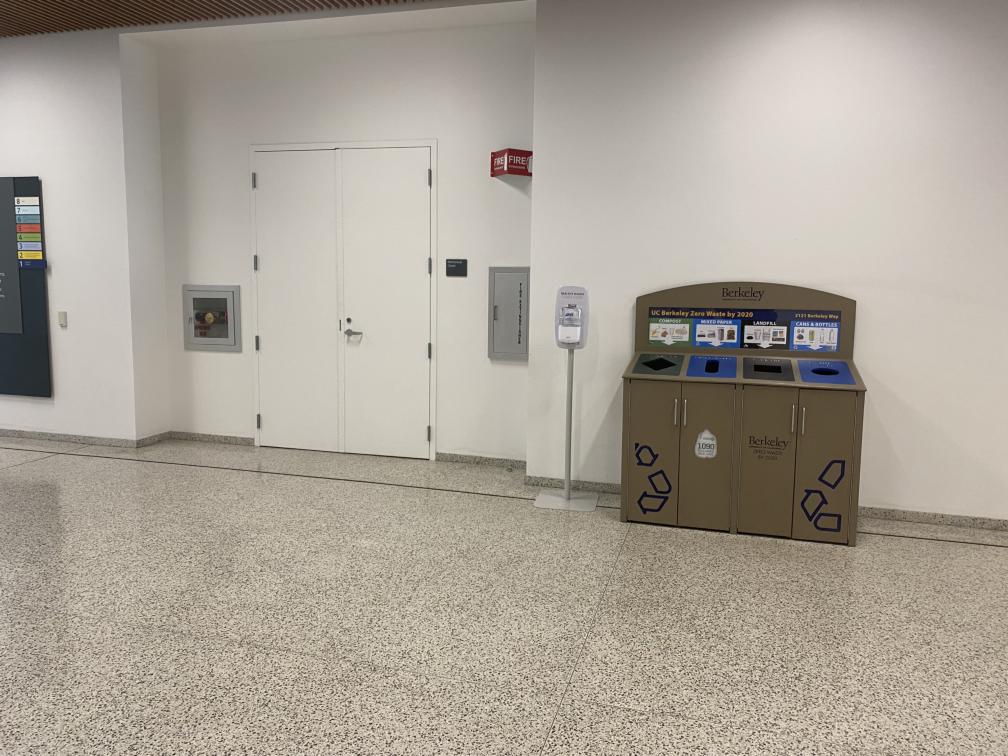
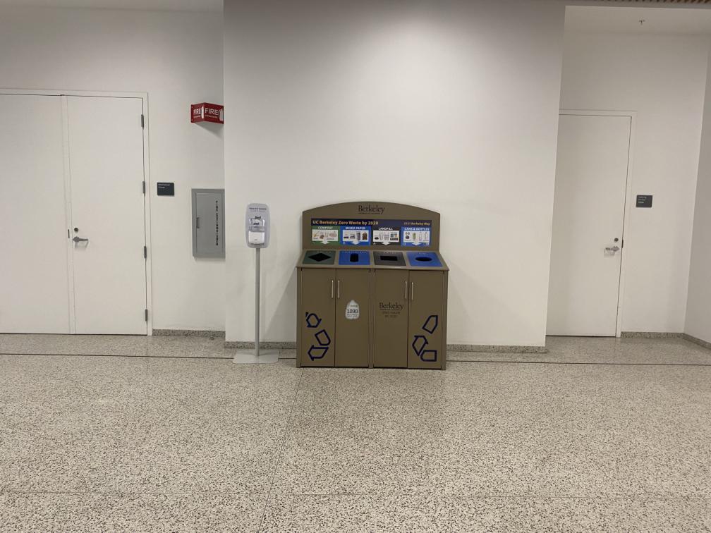
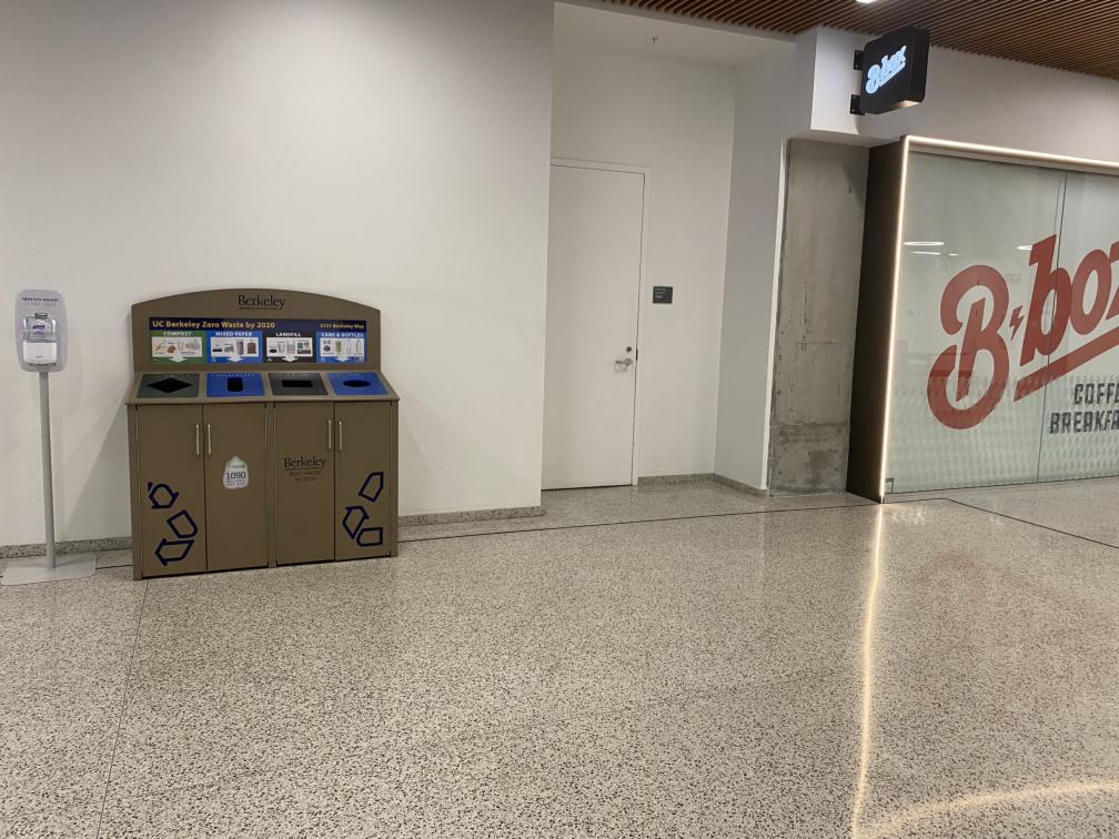
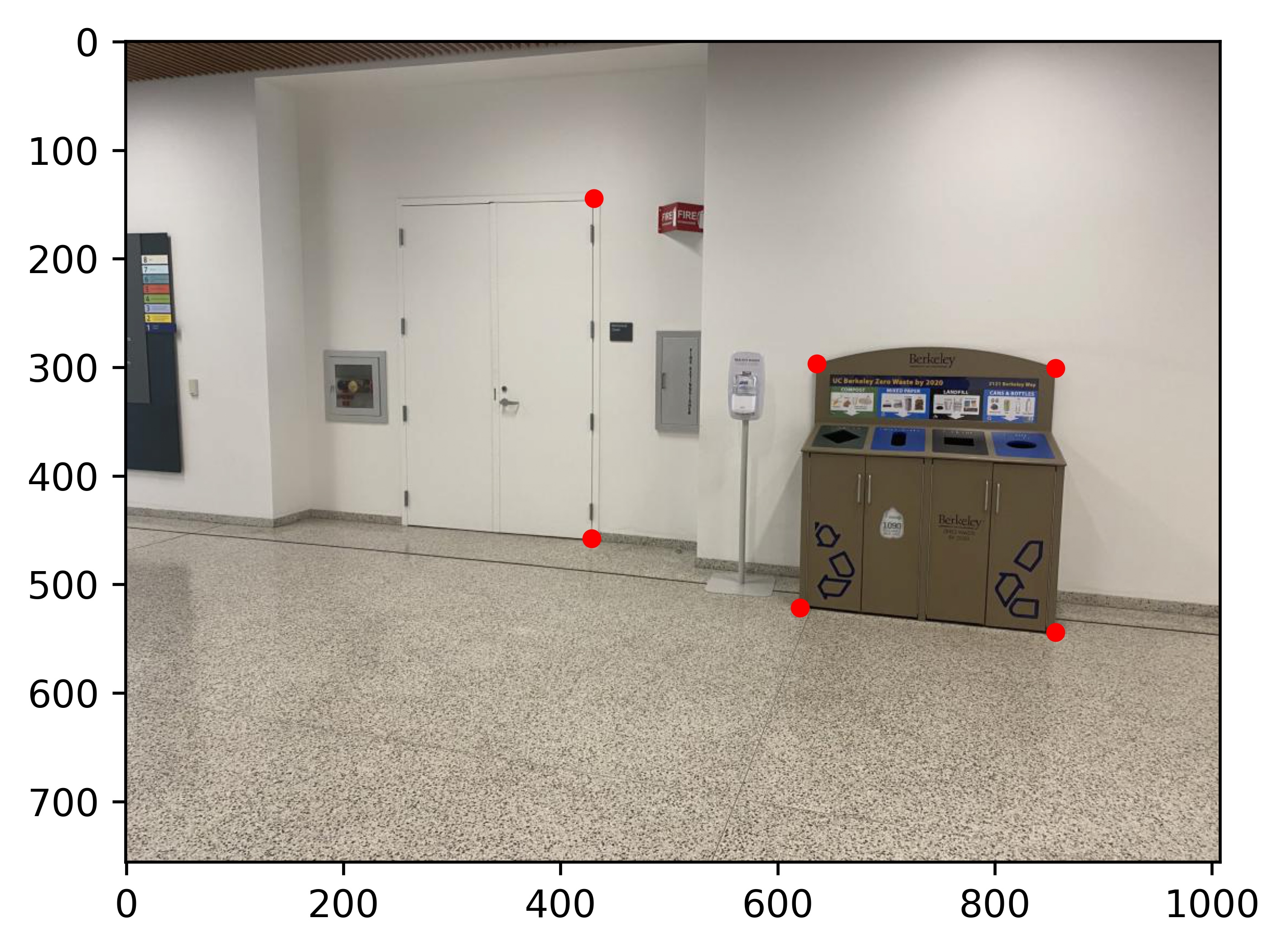
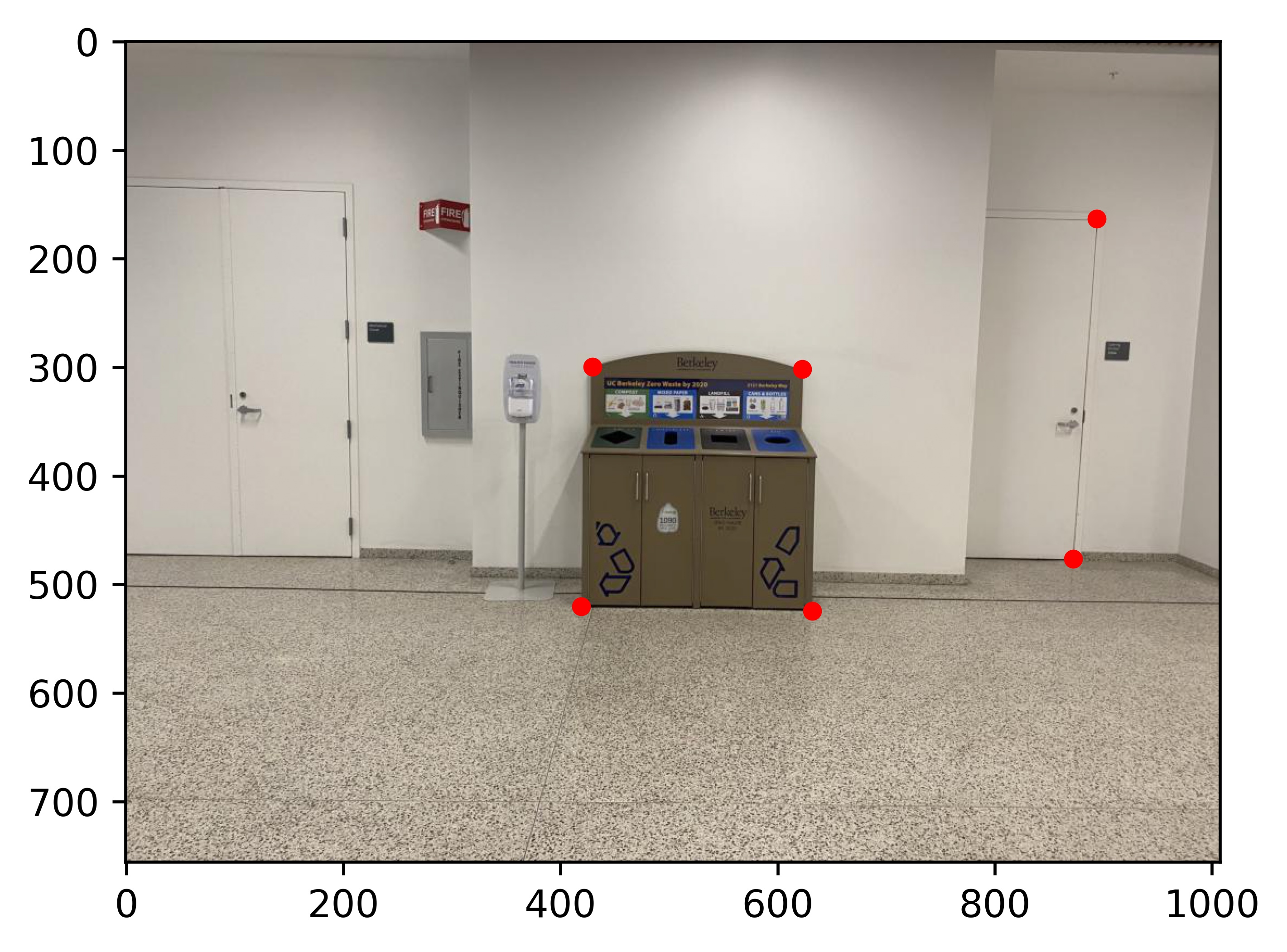
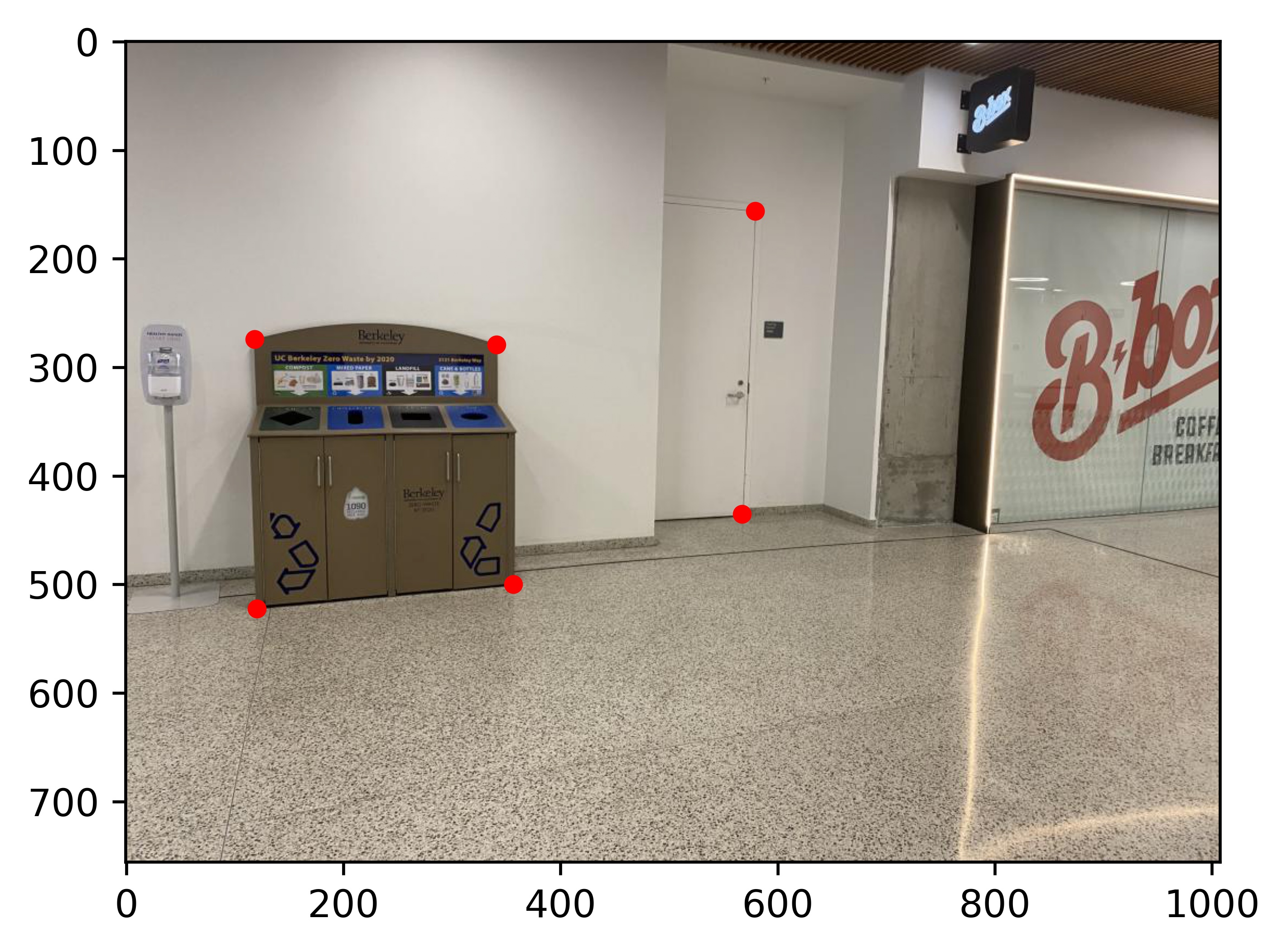
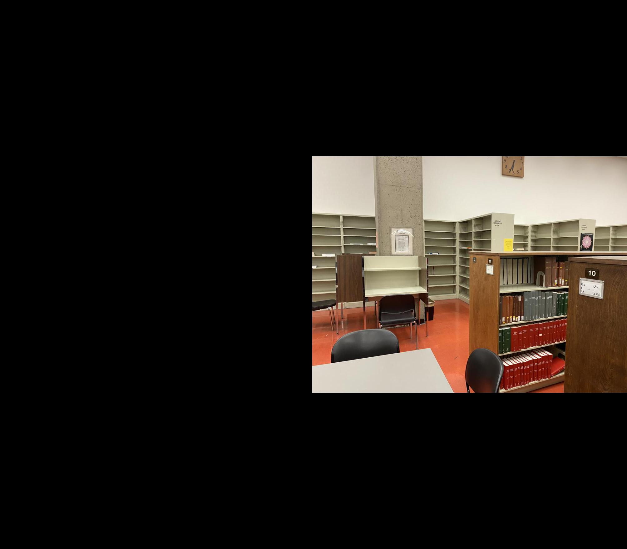
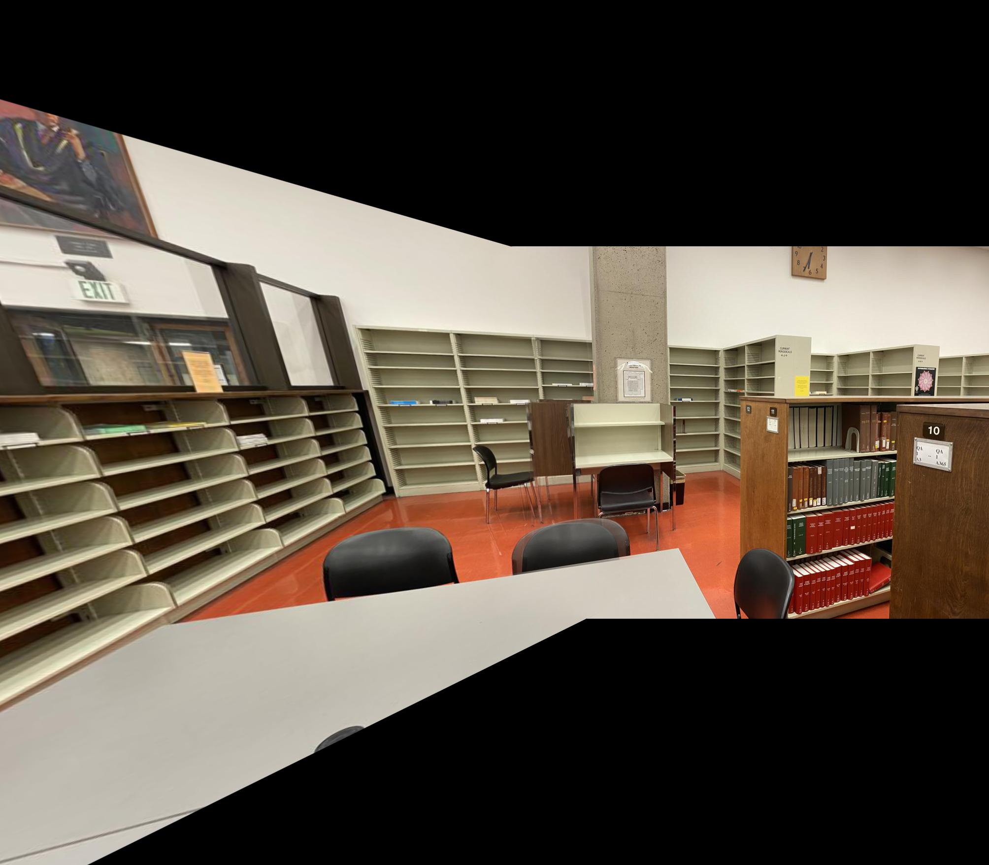
I took the pictures with my iPhone using the AE/AF feature to lock the exposure and focus. I shot a total of three scenes around campus:
Scene 1
|
|
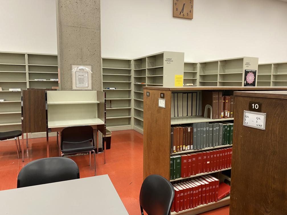
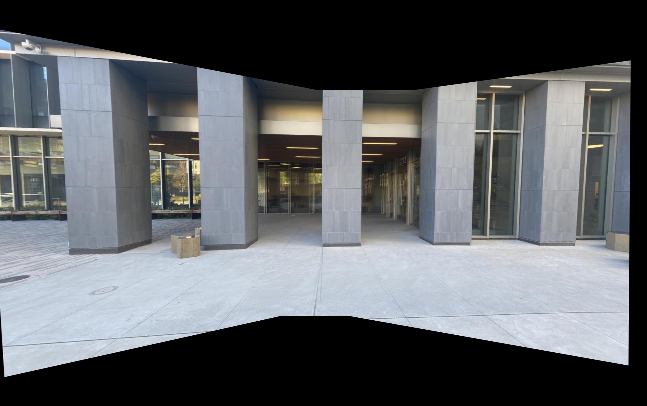
Scene 2
|
|
|
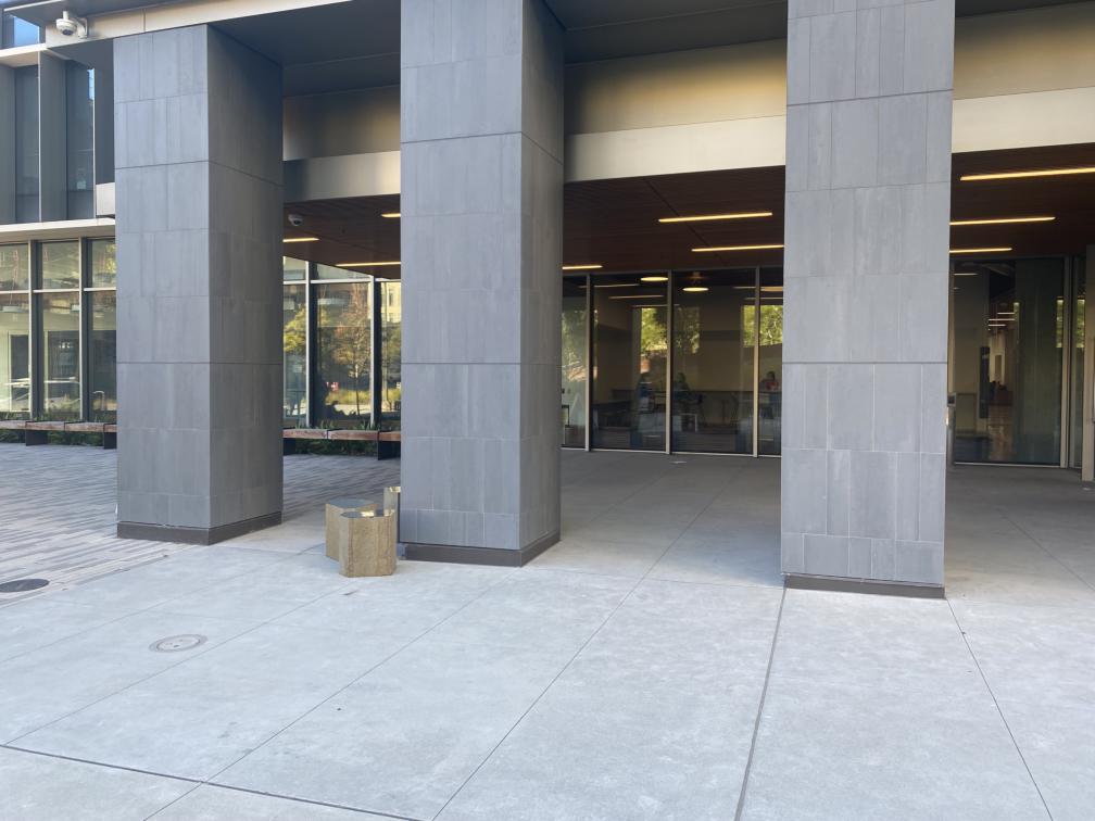
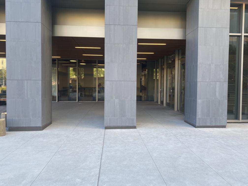
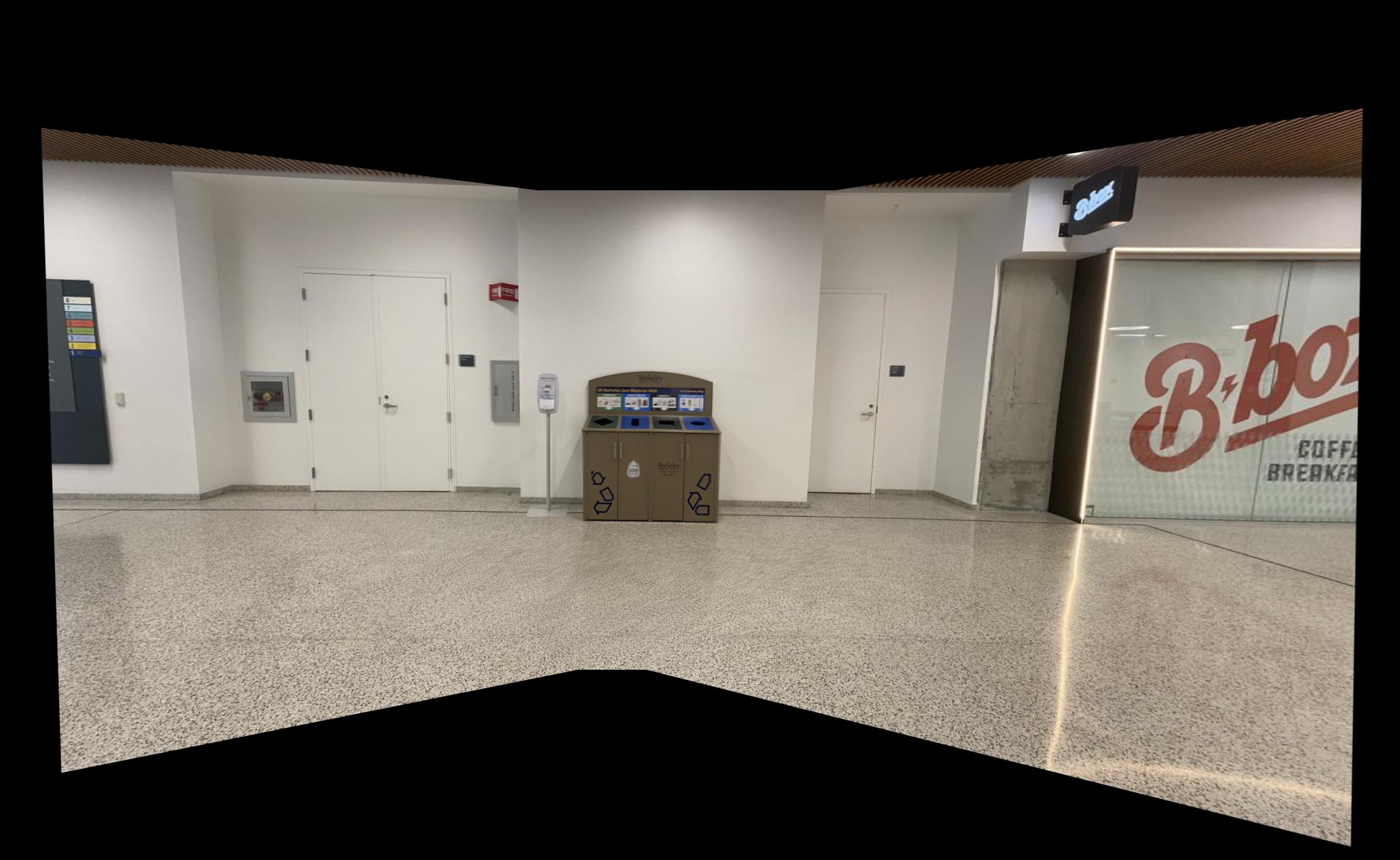
Scene 3
|
|
|
Recover Homographies
We want to recover the homography matrix H such that p'=Hp, where p is the point in the
source image and p' is the warped location of p. We know that the equation satisfies
So H has 8 unknowns. We can solve for the values of H by providing at least 4 correspondences and using
linear least squares. By expanding out the matrix product and substituding w in the first two lines, and rearranging,
we get the following form of a LLS problem Ax=b for n>=4:
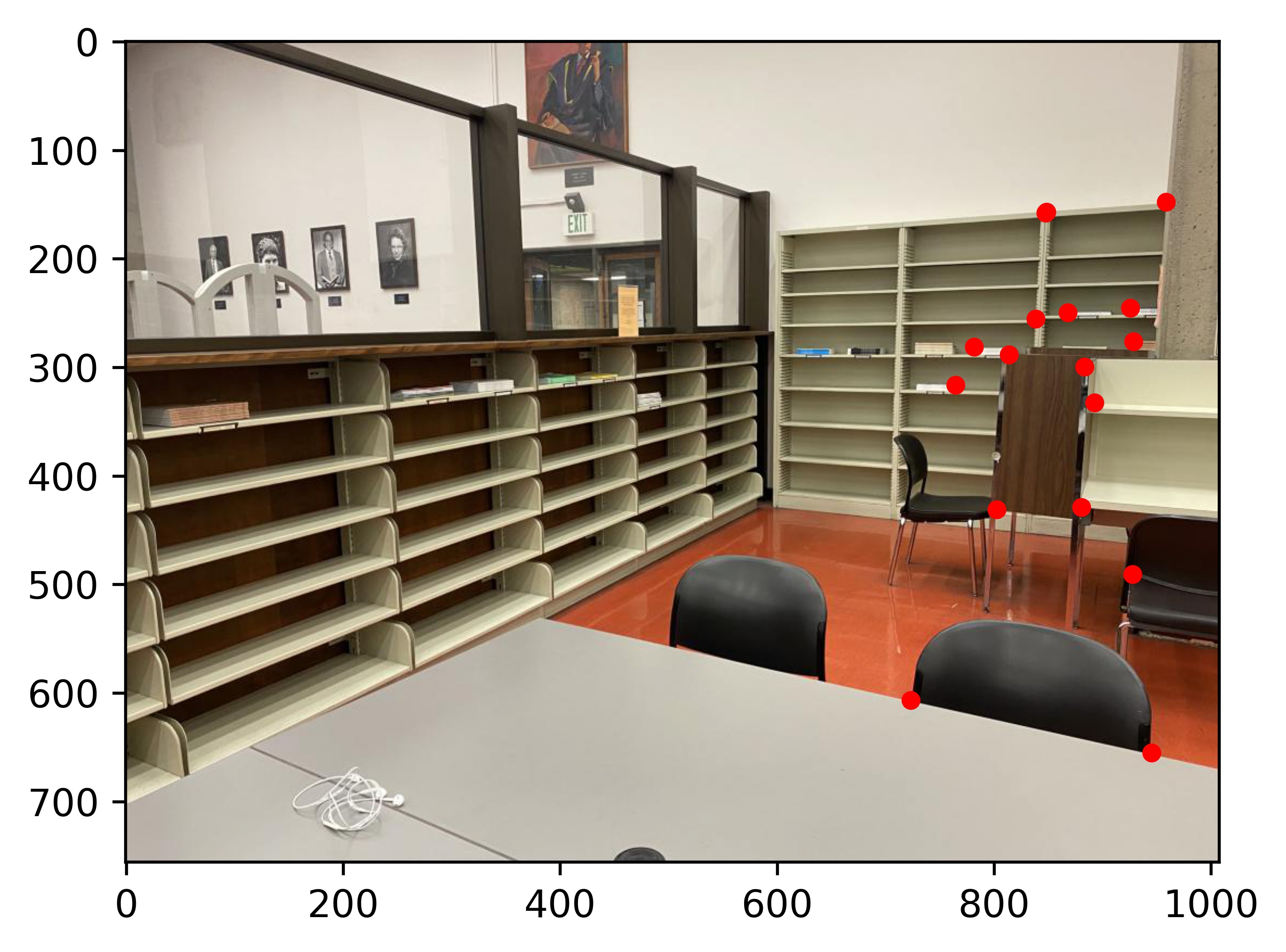
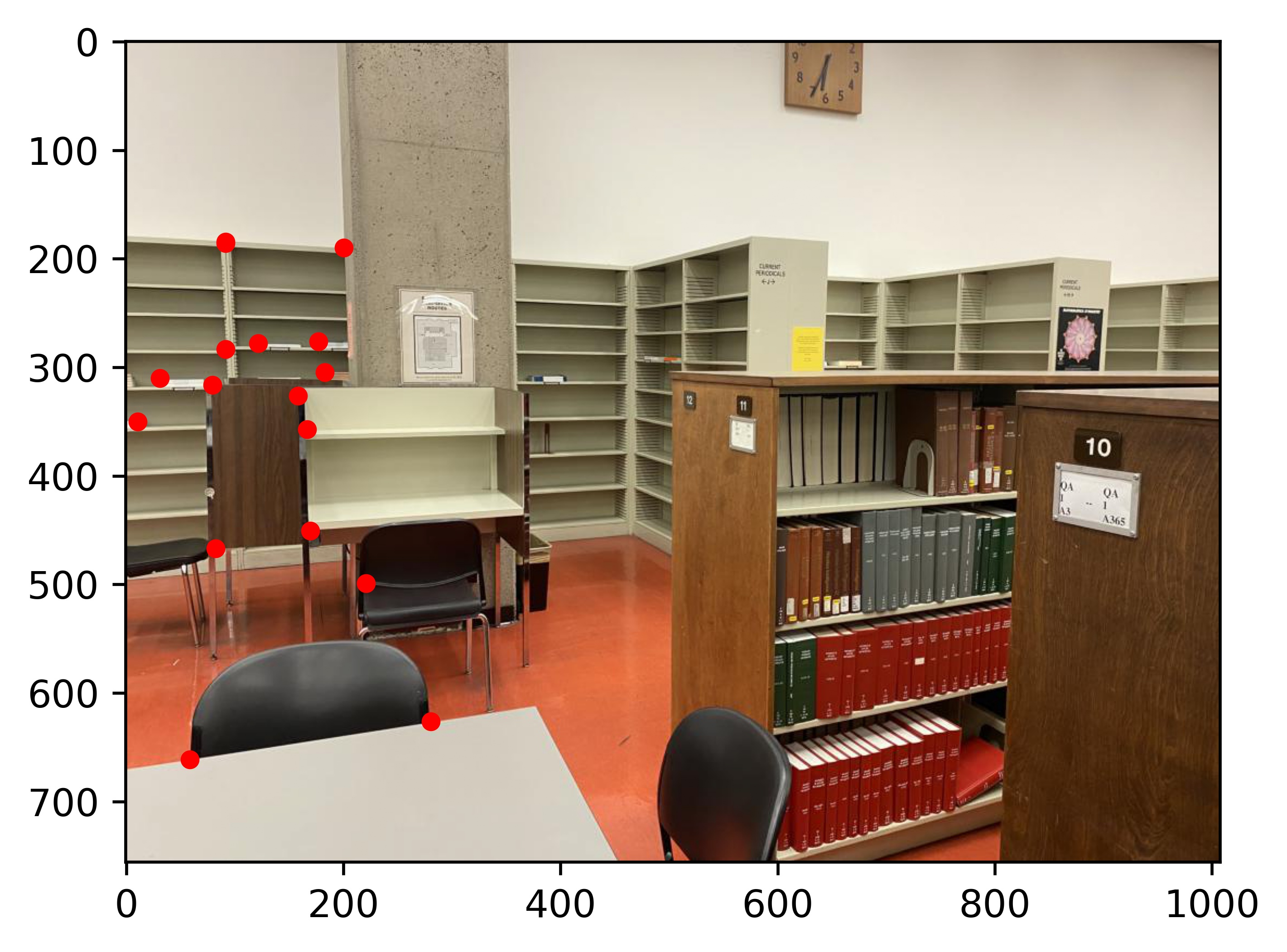
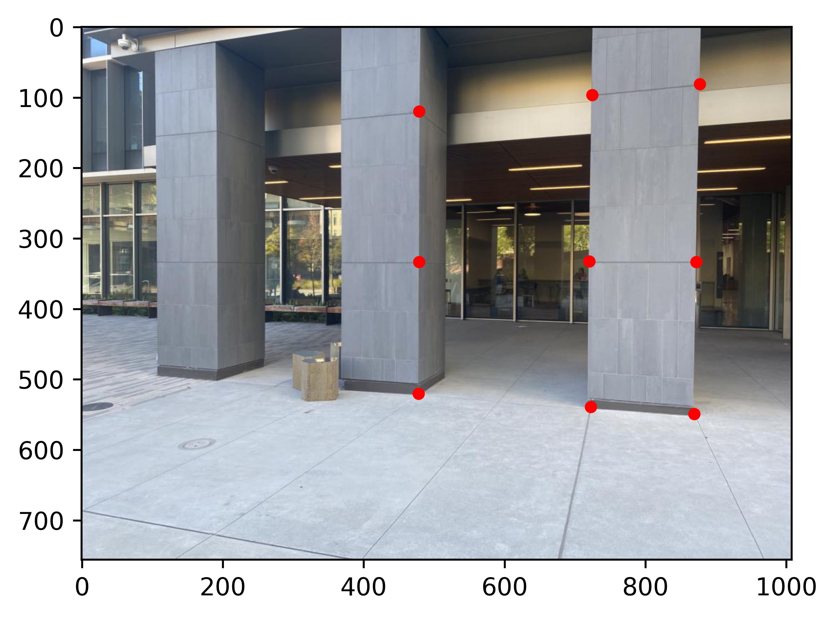
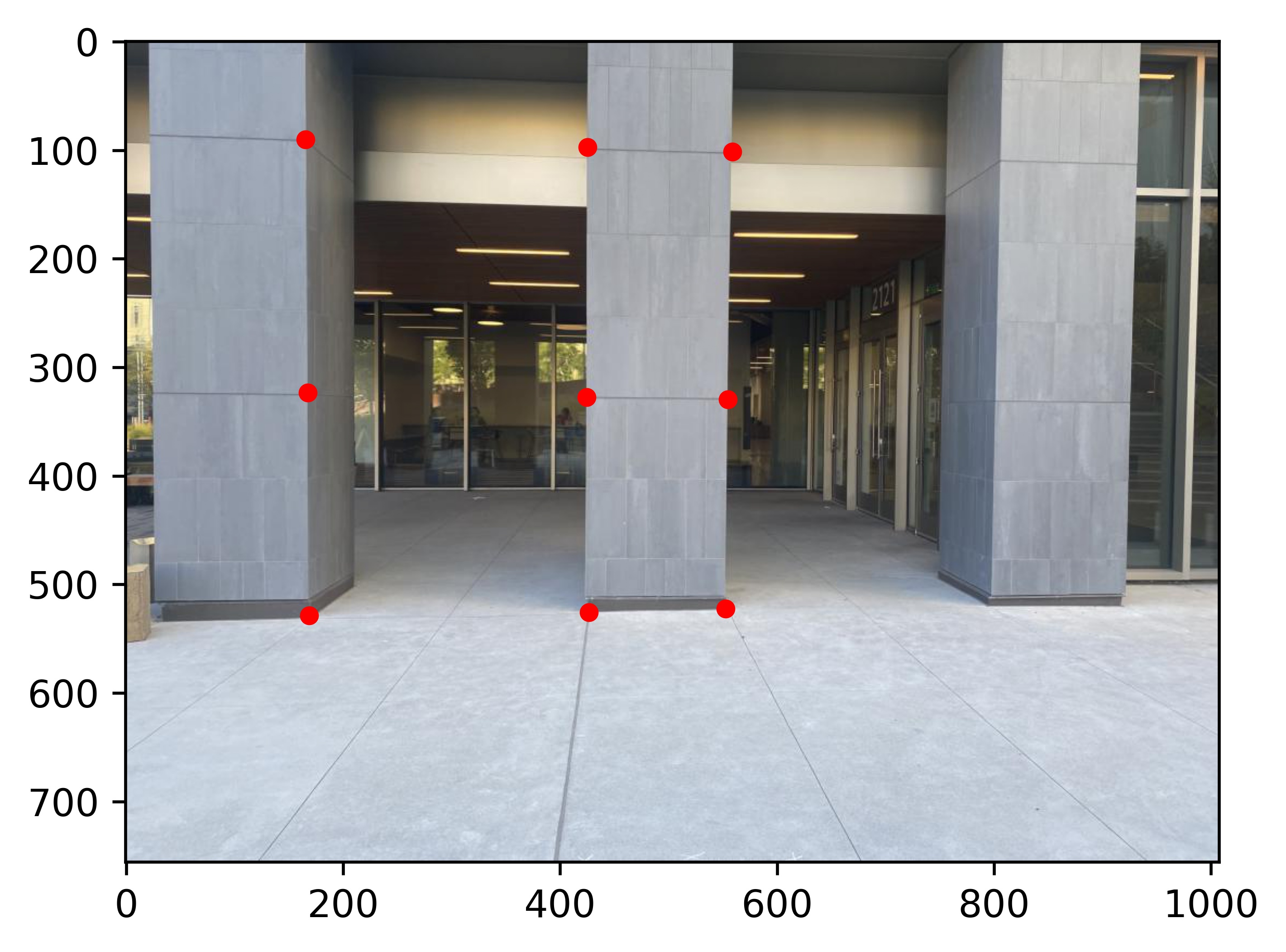
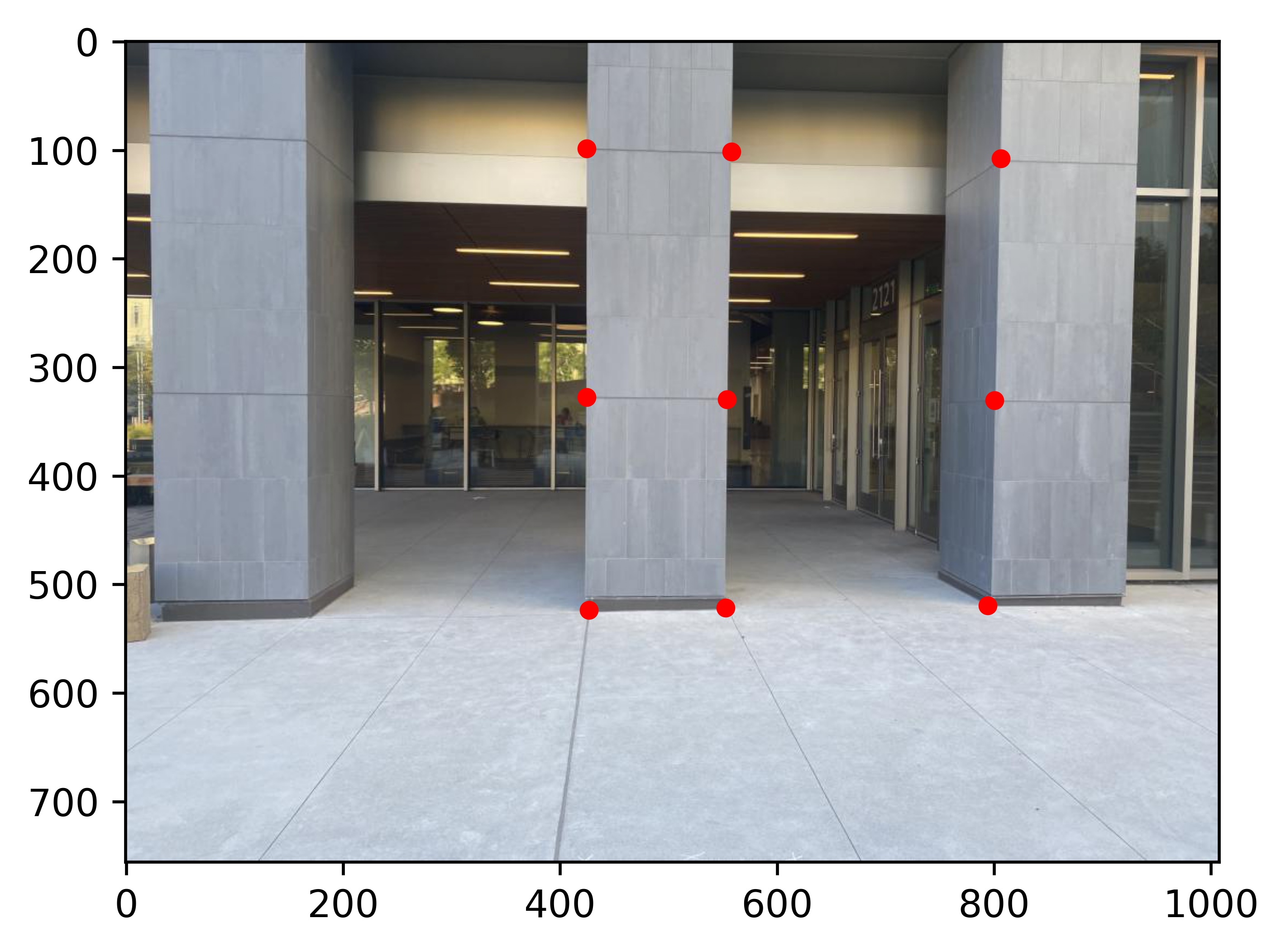
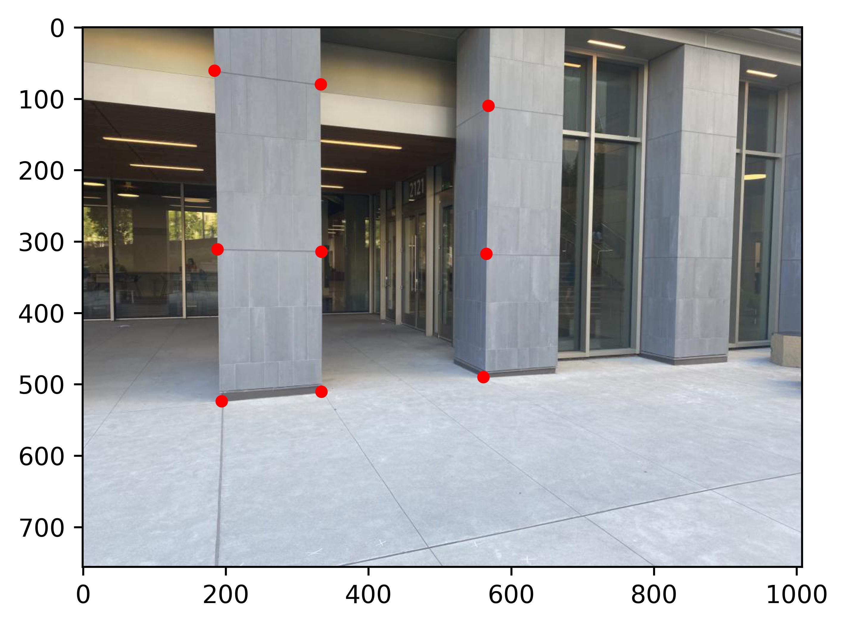
I used matplotlib's ginput to define the following correspondences for each scene:
Scene 1:
|
|
Scene 2:
| Pair 1: | |
|
|
| Pair 2: | |
|
|
Scene 3:
| Pair 1: | |
|

|
| Pair 2: | |
|
|
Warp the Images
For warping the image, I use the inverse mapping method. First, I calculate H_inv. Then I define the target image
as an all black image, and for every single point on the target, transform it using H_inv and bilinear sample from
the source image. For the homography transformation, after multiplying the homogeneous coordinate by H_inv, I have to
divide every element by the last element to get the actual coordinate. In the code, I used OpenCV's remap function to do this
sampling.
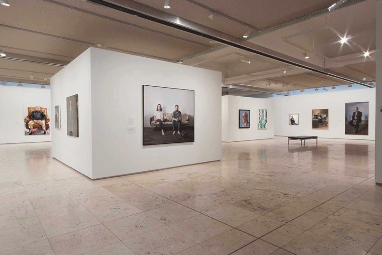
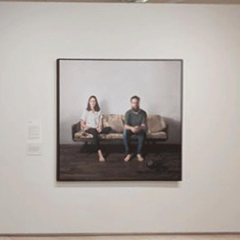
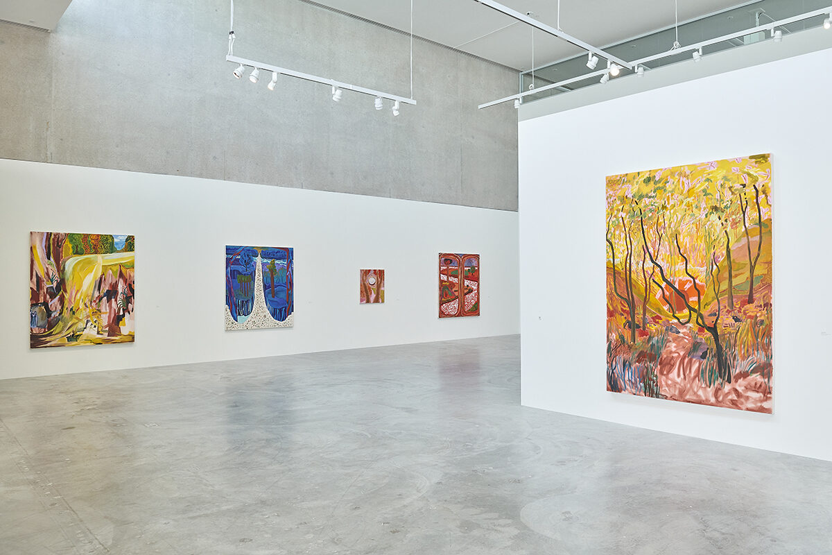
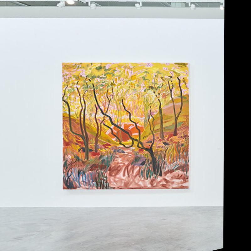
Image Rectification
To test the warp, I took two images of an art gallery, and rectified one painting in each, by selecting the 4 corners of the painting and projecting it onto simply a square in the middle of an 800 by 800 image. We see that my homography and warping are both correct.
|
|
|
|
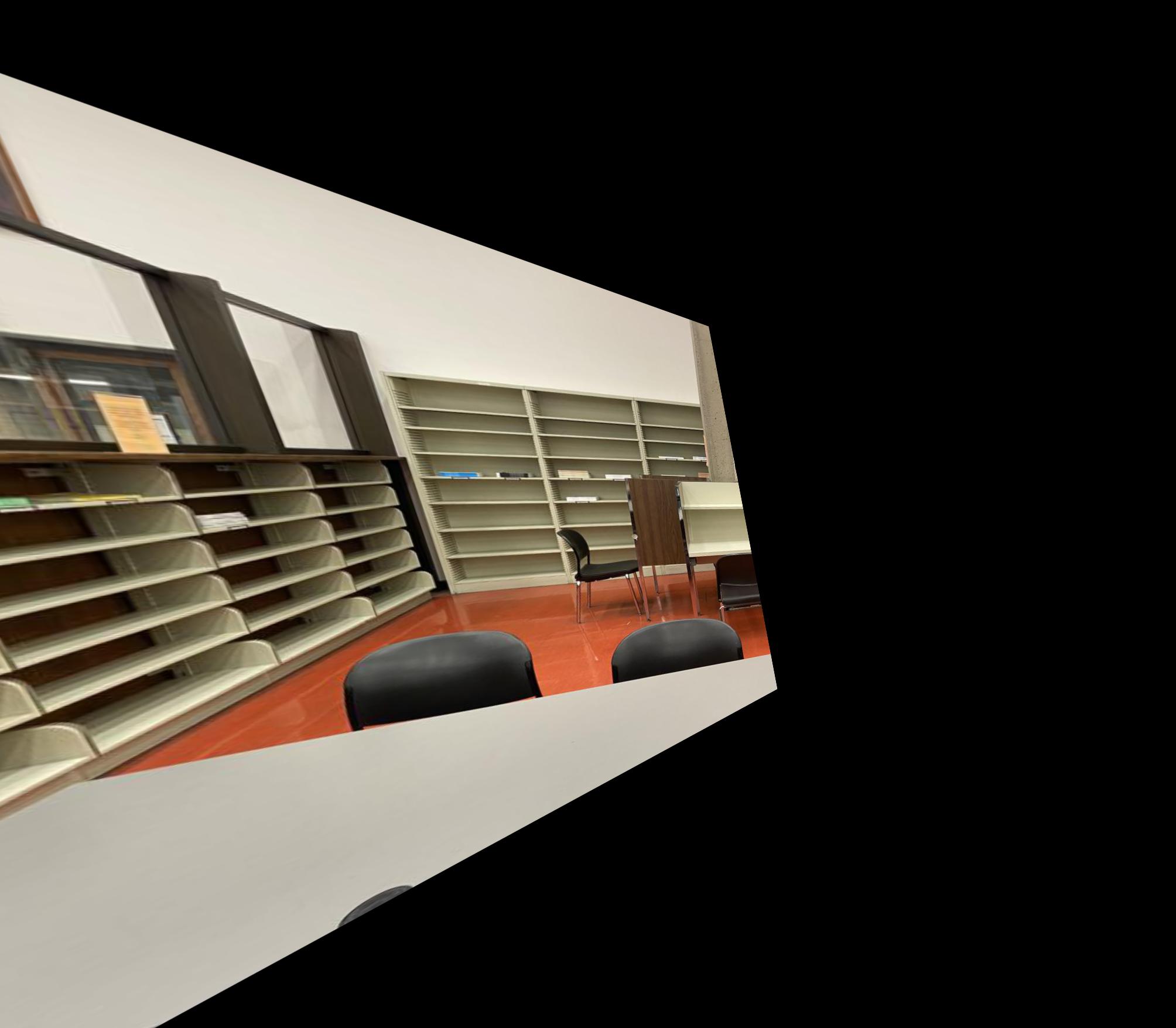
Blend the images into a mosaic
For creating the mosaic, I selected the middle image as the base, and warped every other image to that base image. Here is the step by step procedure for Scene 1. Take the second image as the base. First I padded the base image to the final size of the mosaic:
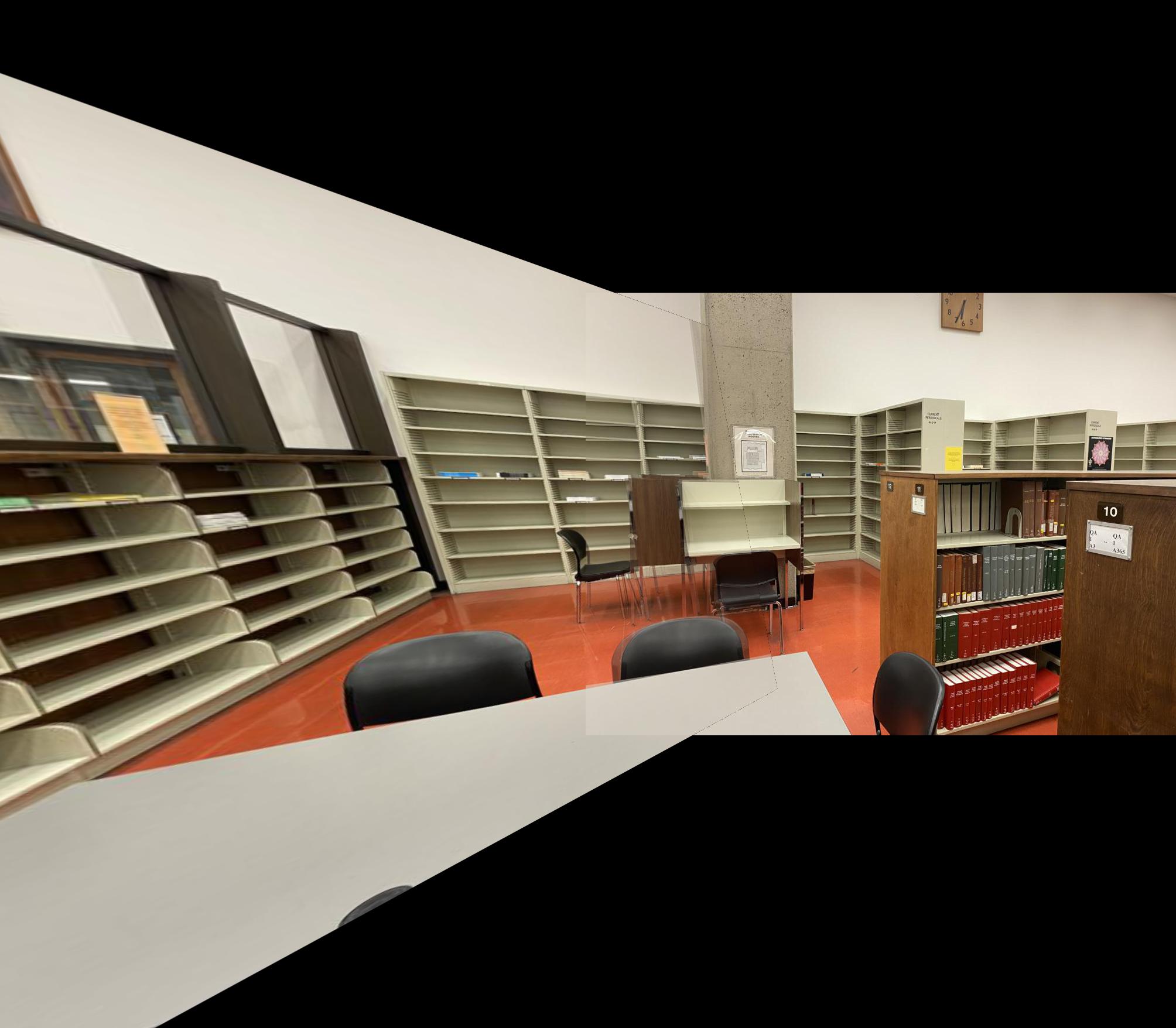
Then calculate the homography from image 1 to image 2 (offsetting the points on the base image by the padding), and warped image 1
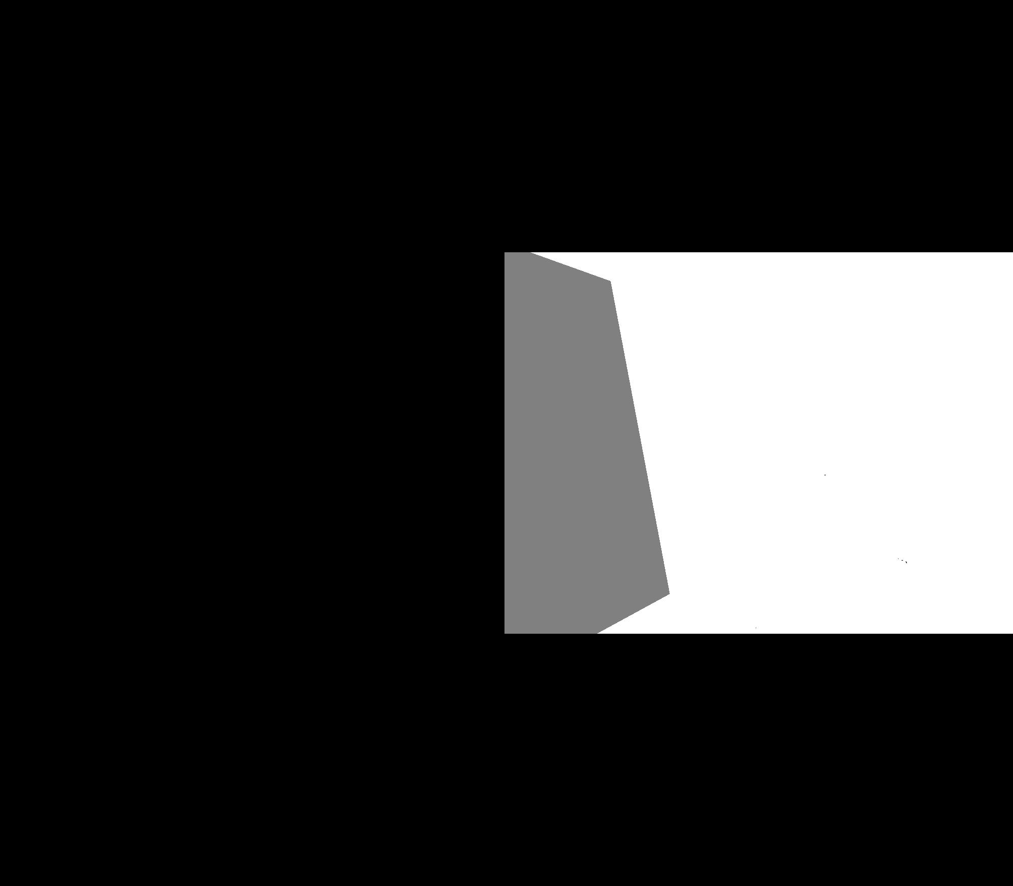
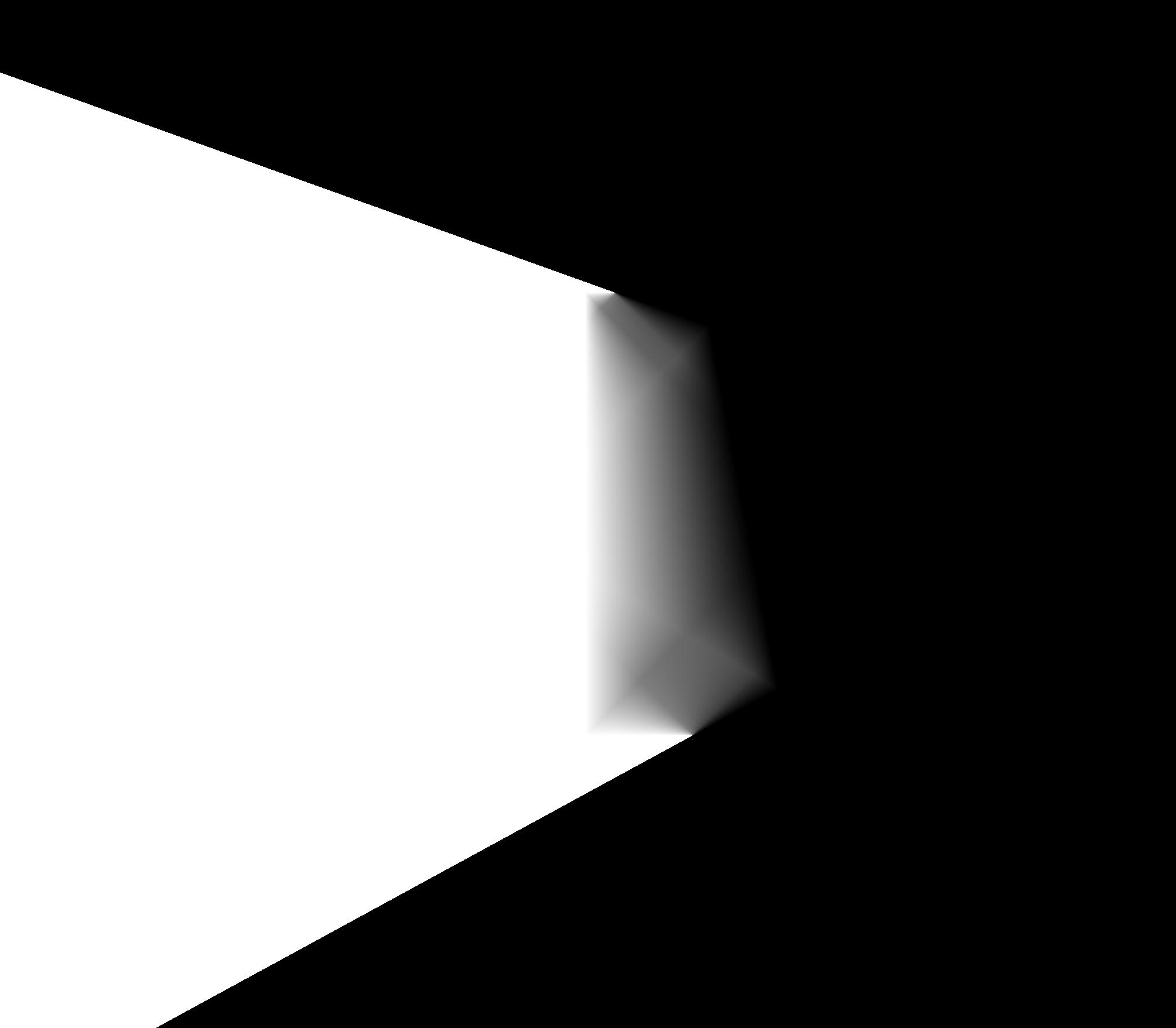
Then, I first naively blended both image with a weighted average using the following mask which has 0.5 at overlapping regions:
|

|
To get:
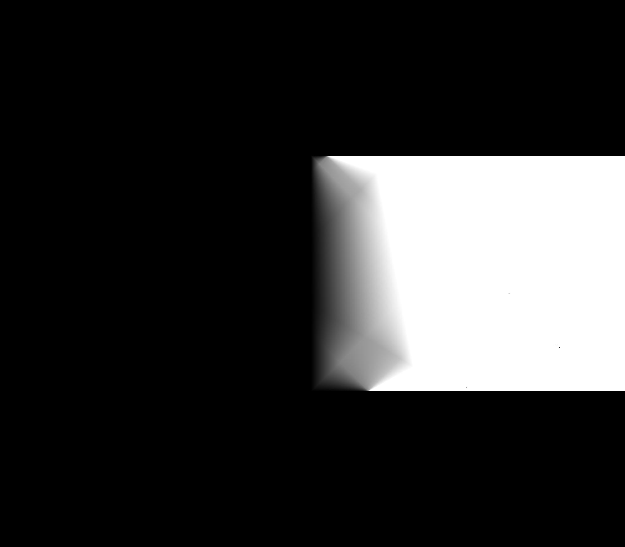
However, we see that the overlapping region has this "ghosting" effect, and we can see the seams very clearly. Instead, use a mask that smoothly blends between one image to the other in the overlapping region, which can be calculated as the ratio of the distance (Manhatten distance is faster to calculate than Euclidean) to image 1 and image 2. As follows:
|
|
This will give us a much better looking blending without any visible seams (on the right):
|
Flat: |
Smooth: |

|
|
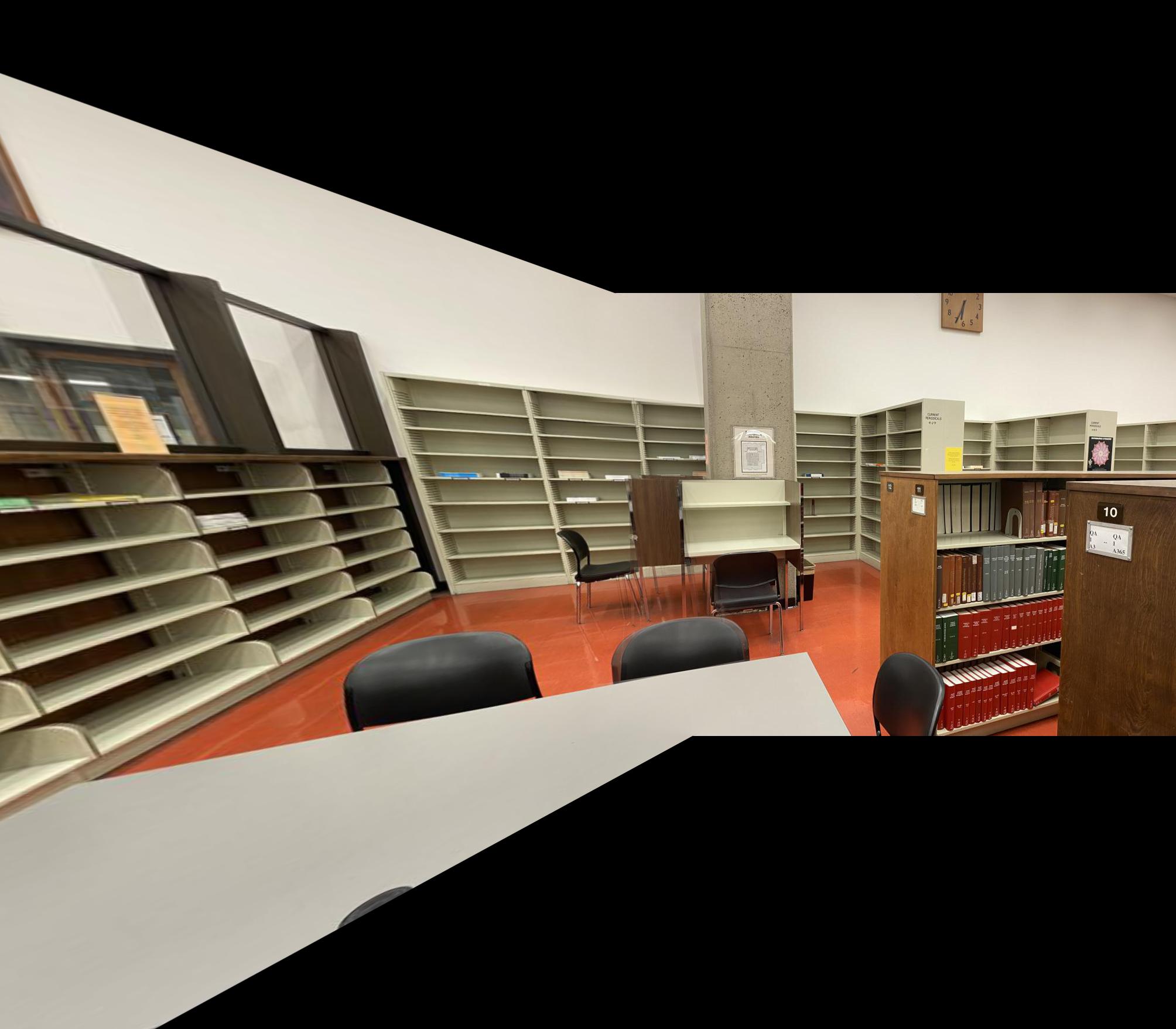
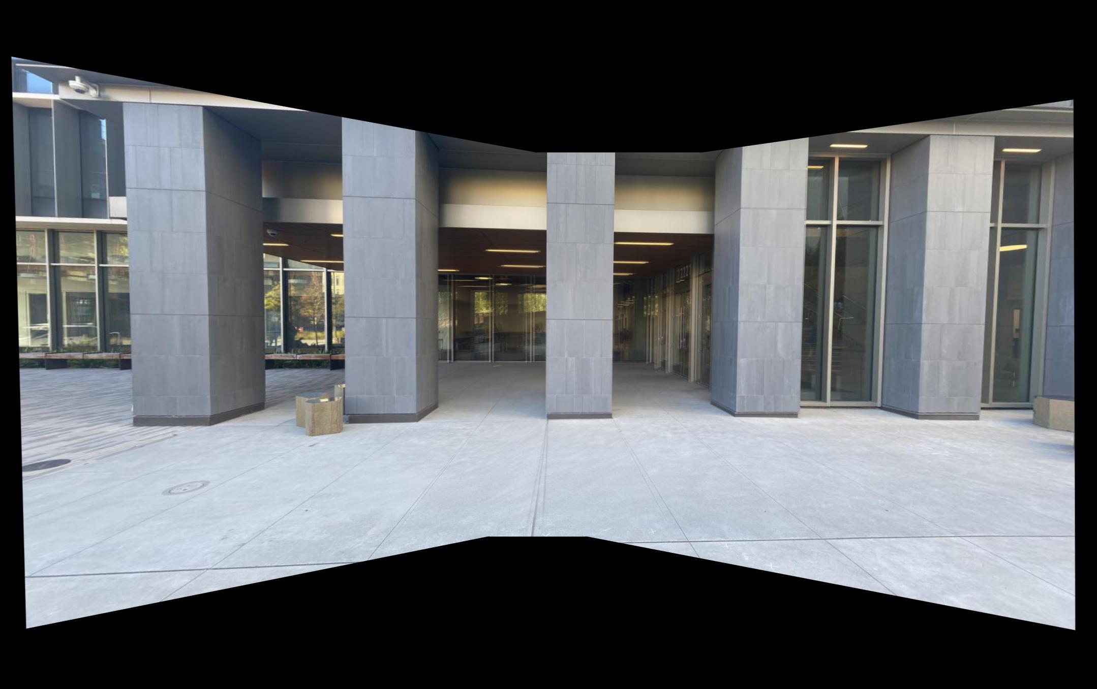
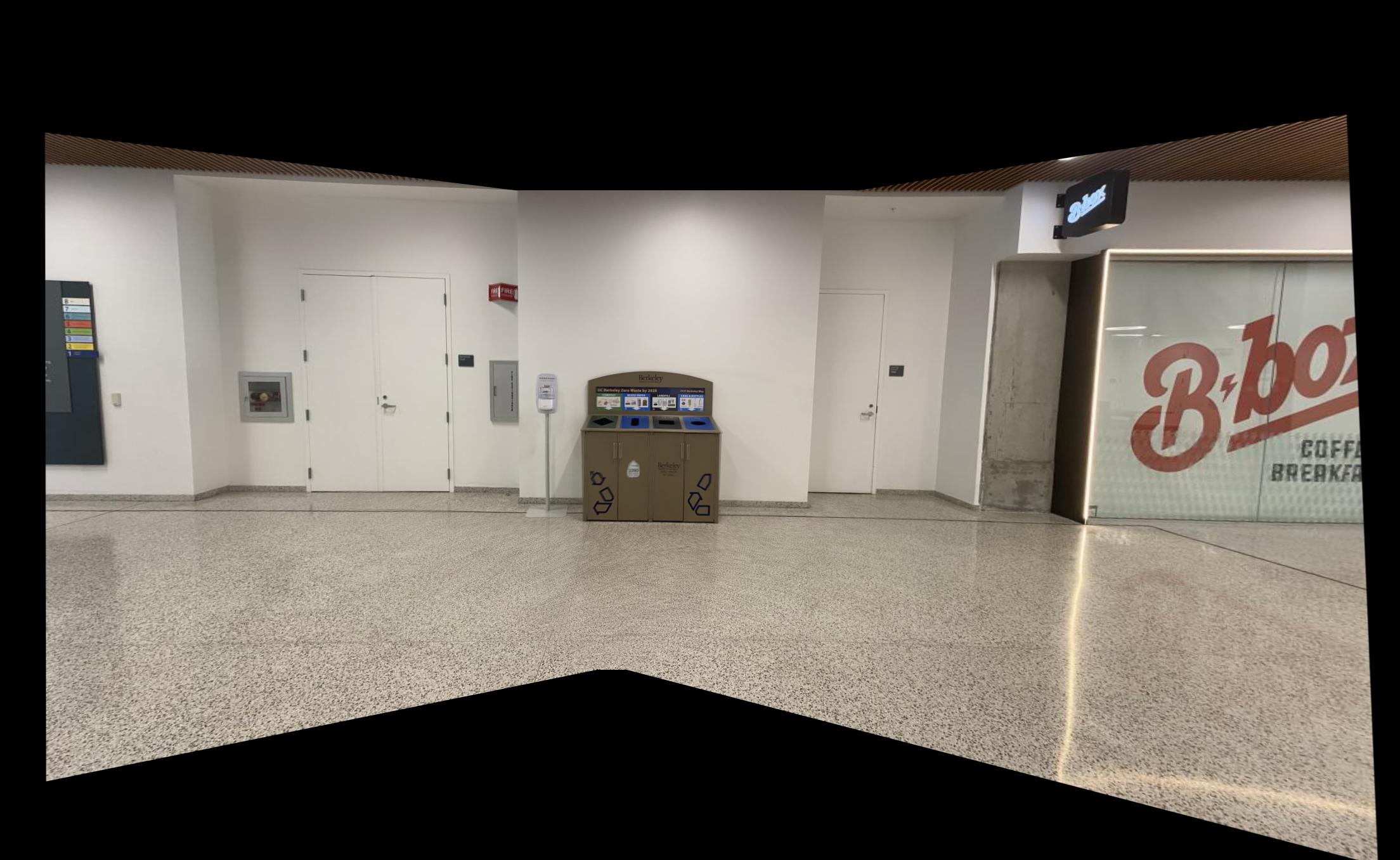
Using the same smooth blending procedure, the following are the results for Scene 2 and Scene 3.
|
|
Part B
Harris Interest Point Detector
In order to automatically align images based on “Multi-Image Matching using Multi-Scale Oriented Patches” by Brown et al, I first start with the provided Harris corner detector. Here is image 2 from scene 1 with the Harris corners:
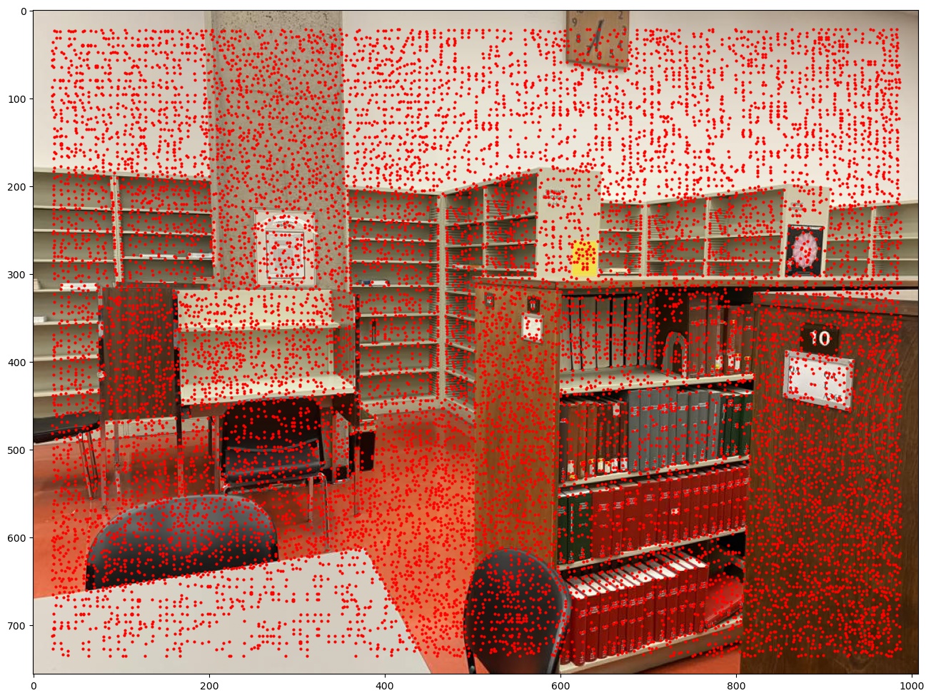
Adaptive Non-Maximal Suppression
We see that there are too many points, so I implemented ANMS to reduce the number of points to only the important ones.
This means calculating a "r" value for each point, which is its distance to the nearest point that has a higher corner strength
(mutiplied by a constant c for robustness), and then getting the k points with the
highest r values. The following is scene 1 image 2 with c=250 and k=250.
We see that most of the points are interesting points in the corner, with some in the white background.

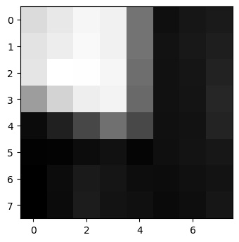
Feature Extraction
Next, I extracted a feature vector for each point, which is just a 40x40 patch around each point downscaled to 8x8 for anti-aliasing. Here is an example feature:
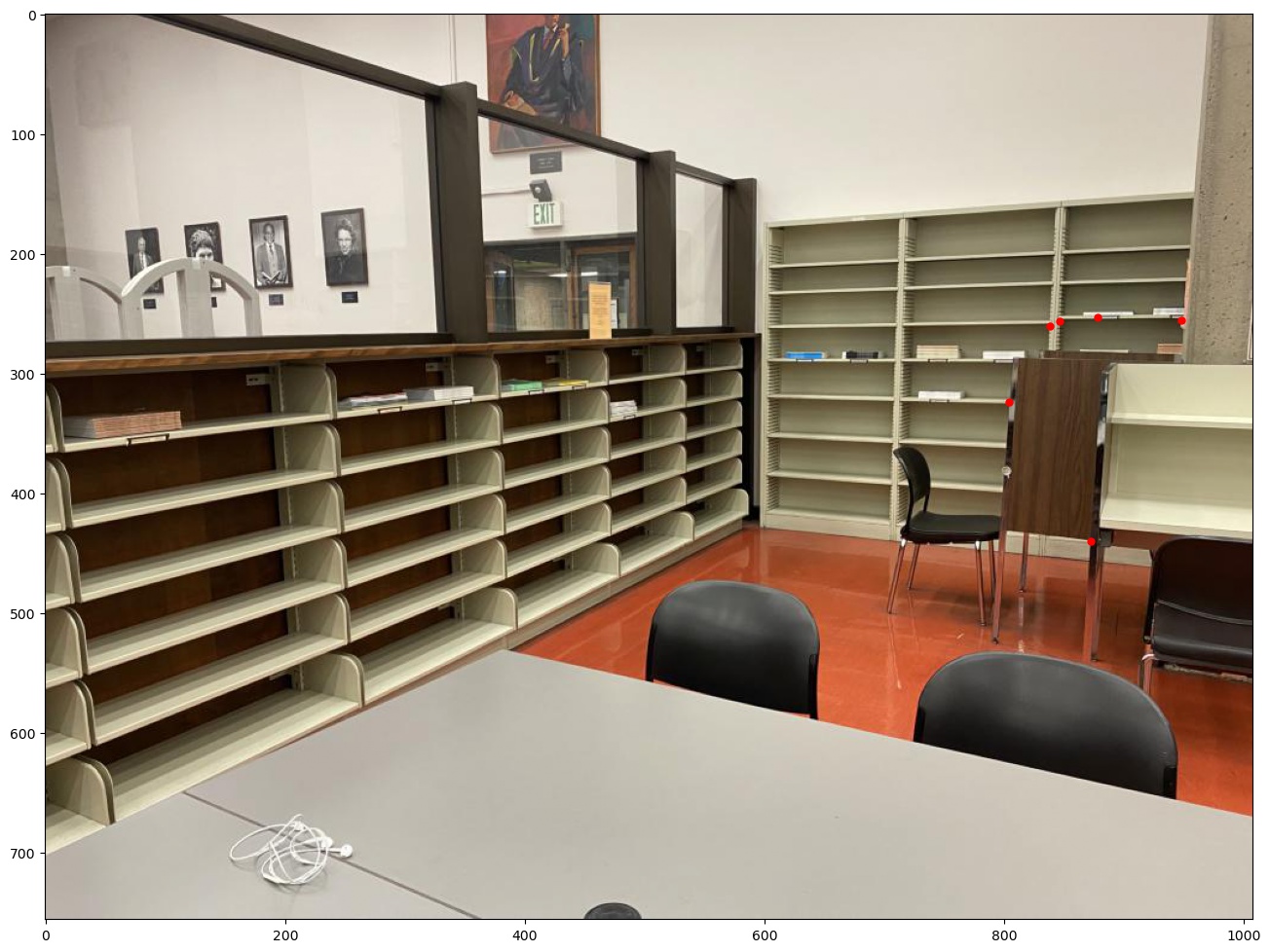
Feature Matching
Then I matched the features of two images by taking each feature from one image and finding the SSD with every other
feature, then calculating the Lowe error estimate of 1-NN/2-NN (the one with smallest SSD divided by the second smallest SSD),
and then only taking the ones with error below some threshold=0.4
Here is an example matching between the two images from scene 1 (ANMS params of c=0.8,k=250):

|

|
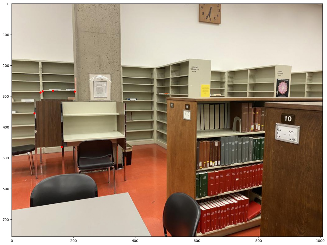
RANSAC
We see that there are some points that don't actually match. This is okay because we will filter one last time using RANSAC
to find the homography matrix. I do this by randomly sampling 4 points each iteration to calculate H, then
transforming all points using H and only keep the ones with an error of less than some eps.
This is called a consensus set, and after some n iterations we use the largest set to estimate H
one last time. Here is an example using scene 1 and eps=0.5, n=8000, we get the following points:
|
|
All Together
Here are the three scenes stiched together comparing between manual (left) and automatic (right). We see that the automatic stitching does comparably with my manually tuned points.
|
Manual: |
Automatic: |
|
|
|
|
|
|
|
|
|
What have you learned?
The coolest thing was how well the automatic stitching worked. I spent lots of effort choosing points to make all the homographies look really good, and the algorithm just does it automatically.