Autostitching Photo Mosaics

In the first part of this project, I explore rectifying images to a different perspective and creating mosaics using homography matrices. In the second part, I look into how to stitch images automatically.

Part 1: Image Warping and Mosaicing

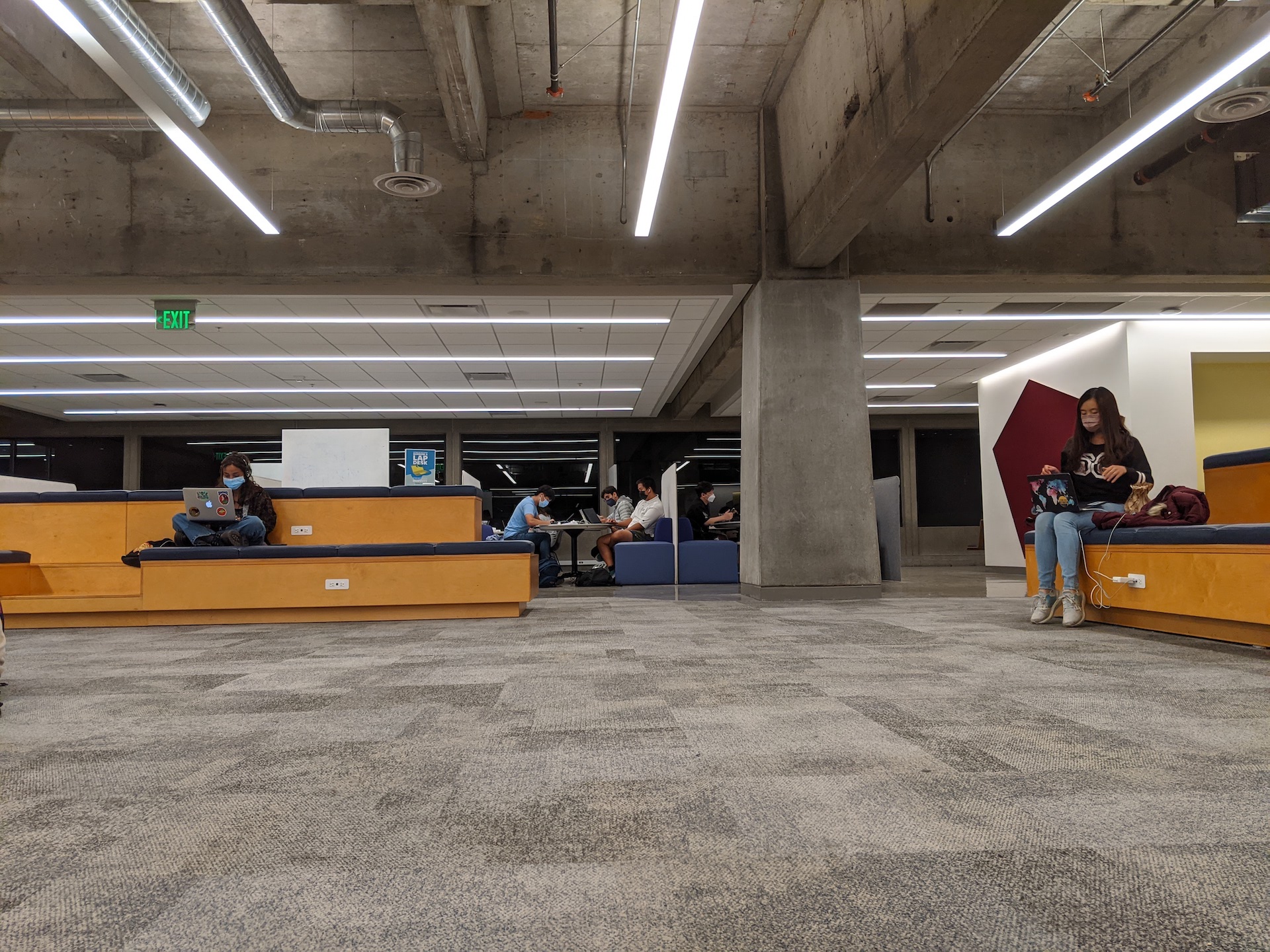
Shoot and Digitize Pictures

To rectify images, we simply just take pictures of an object. In order to stitch images together, we first take pictures from the same spot, and rotate the camera so that each image shares key features. This is so that we can later recover homographies for the matrix and stitch them together.

Recover Homographies

To project an image onto a different plane, we first need to find a homography matrix. The homography matrix is a 3-by-3 matrix that can be solved for by the equation Ha = b, where H represents the homography matrix, a are the coordinates that we want to transform, and b are the coordinates of the image we want to transform to. We then select 4 points in the image, as our homography requires 8 unknowns (4 from the source image, and 4 in the target image). Four points correspond to the image we select the points from, and the other come from the square that we project the image on. When we rectify images, we project images onto a 500-by-500 square. When we stitch images together, we select at least 4 points from a source image and at least 4 points from a target image (in our case, we select around 12 points for each stitching). We then use least-squares to solve for H given an overdetermined system. The system of linear equations for our least-squares problem can be shown in the following equations (inspired by this website)

Warp the Images

To warp the images, we first transform the corners of the image using the homography matrix. We then find all the points within these transformed corners, and interpolate the color at these points from the original image.

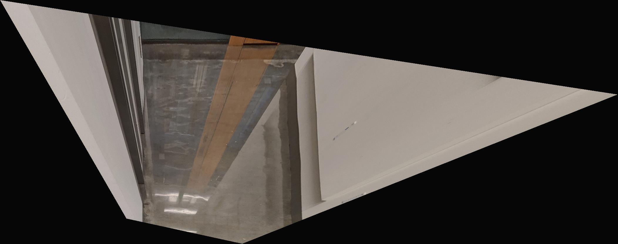
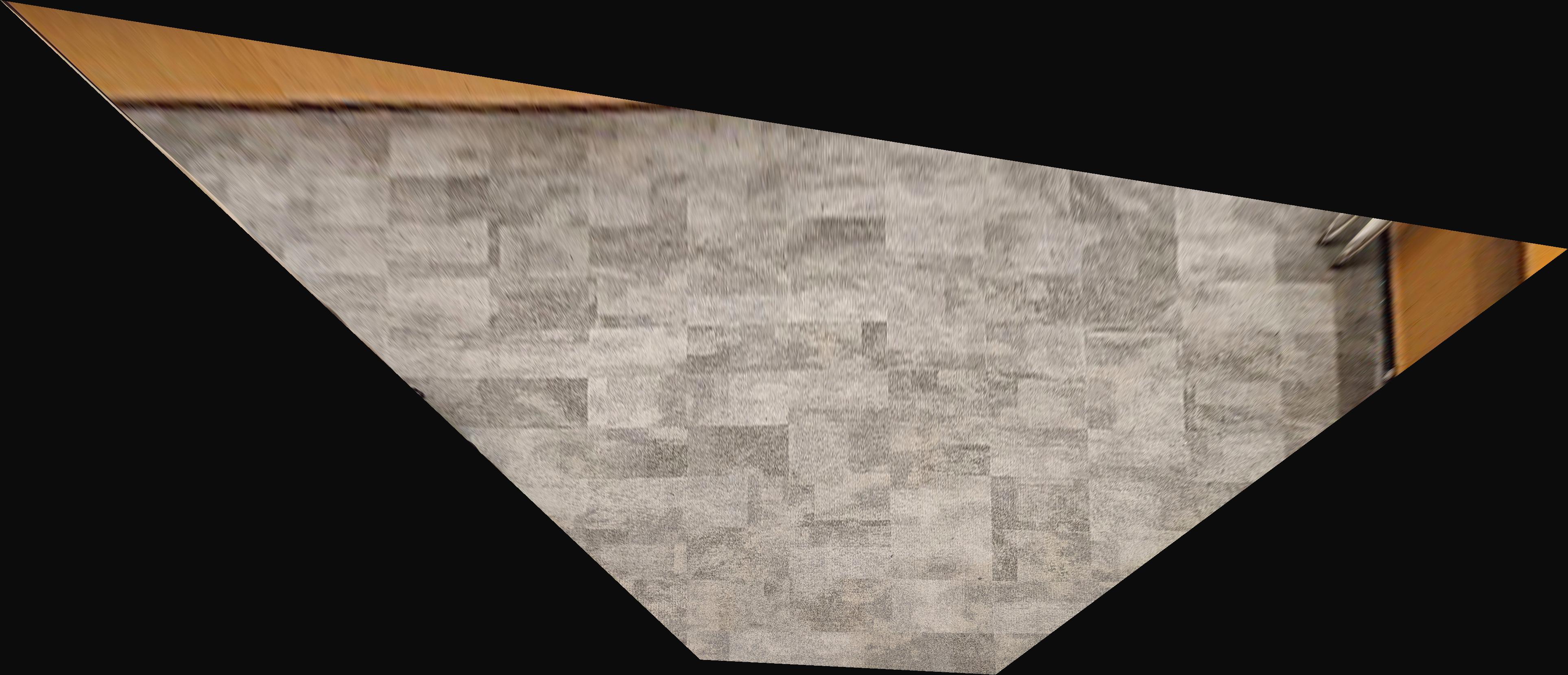
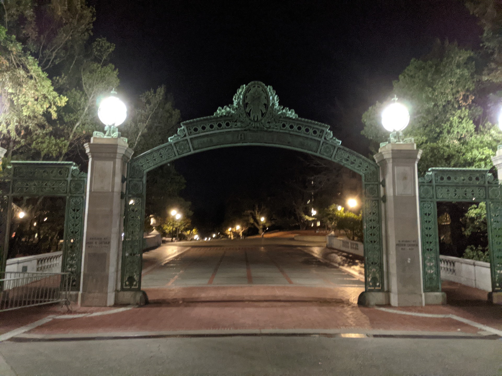
Image Rectification

To rectify images, we select four points in an image, and project use these points to project the image onto a 500-by-500 square. Here is the result of the rectified images:

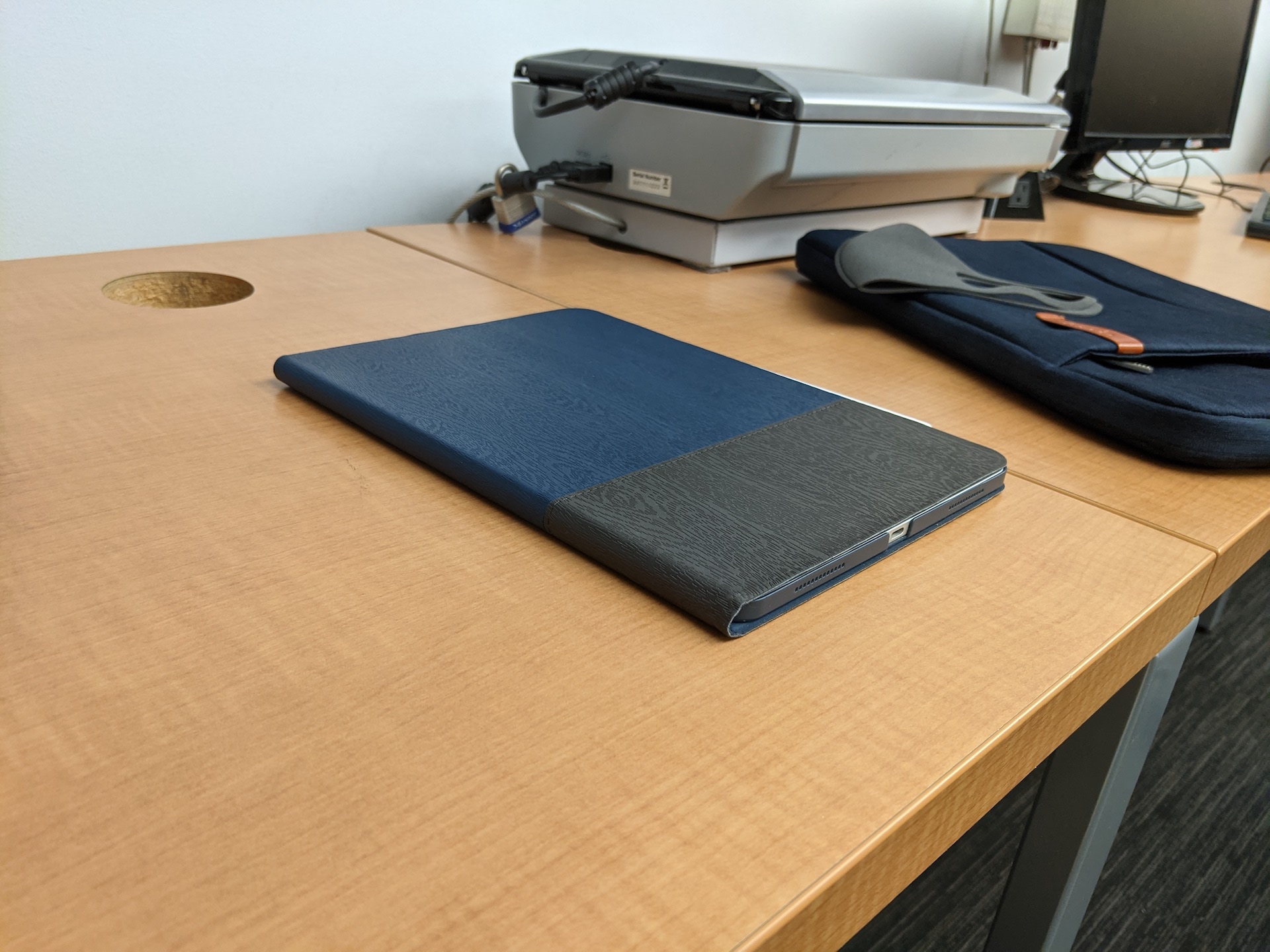
iPad

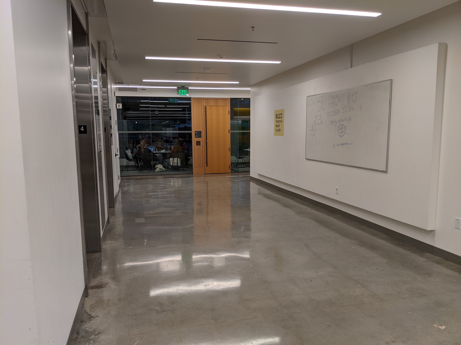
Moffitt Hallway

Moffitt Floor

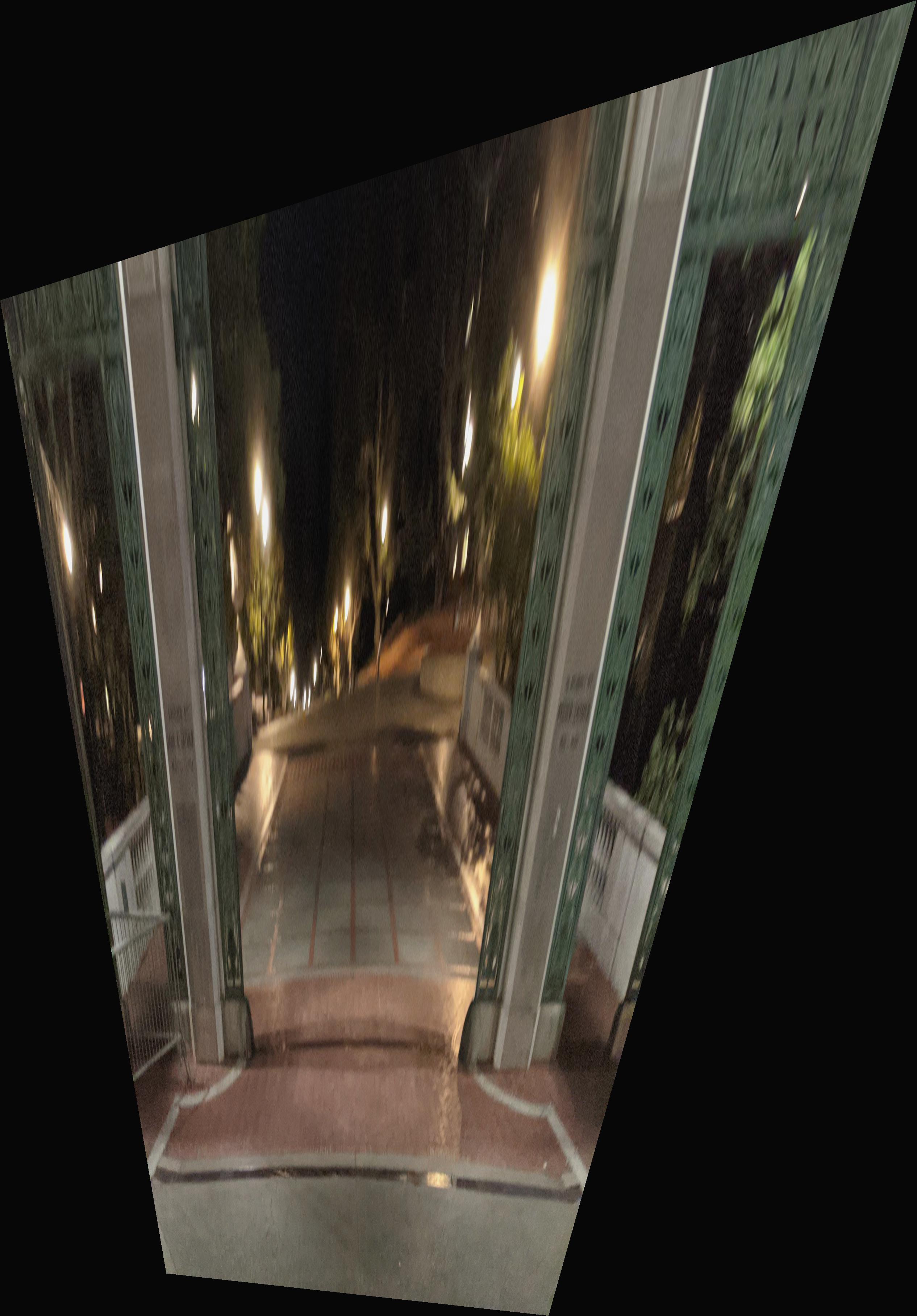
Sather Gate

Blending Images into a Mosaic

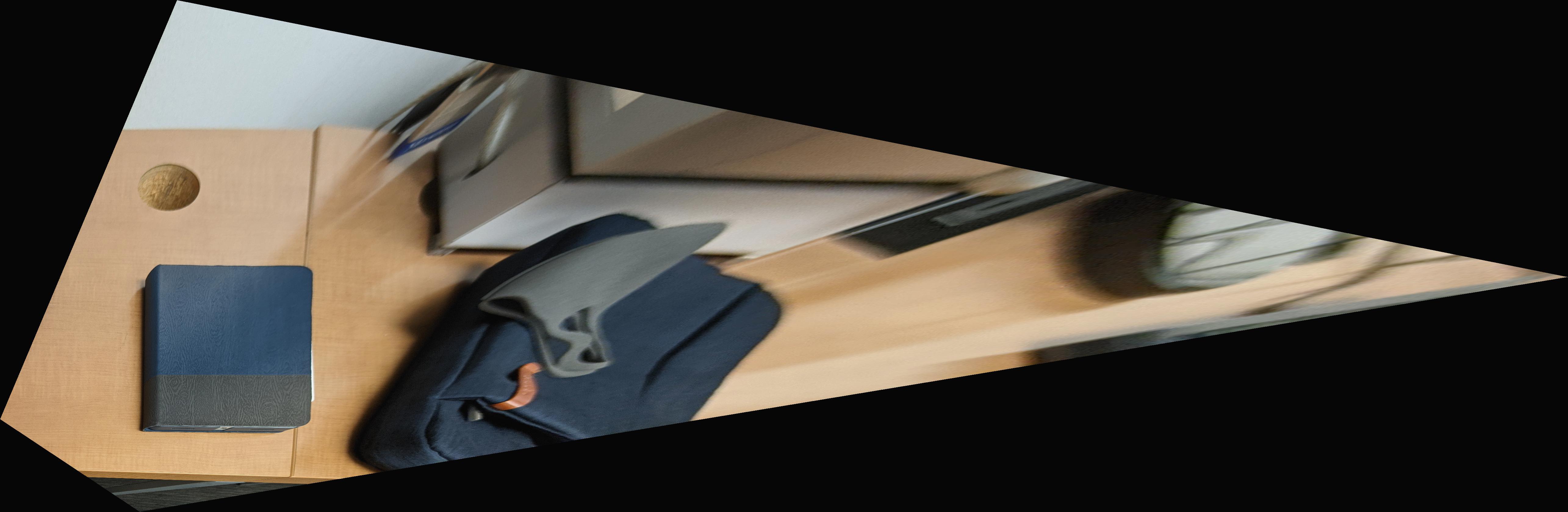
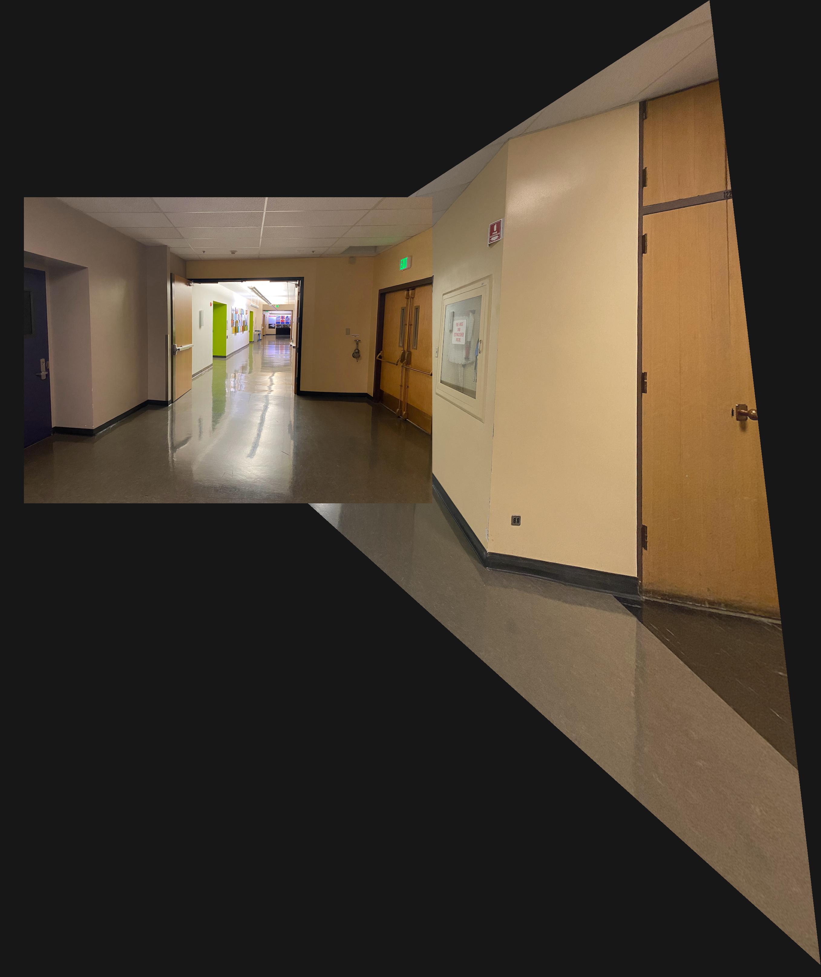
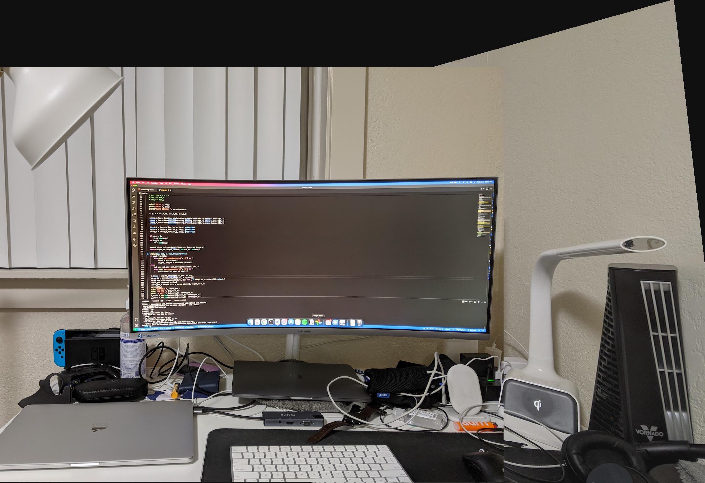
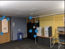
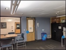
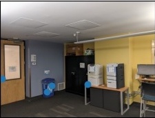
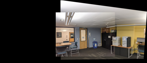
We take the images that contain overlapping key features, and project one image on to the other image. In order to do this for multiple images, we start with the left-most image, and project all other images onto the left-most image. We then align the images with each other, and we can blend the images using a weighted averaging. Here is the result:

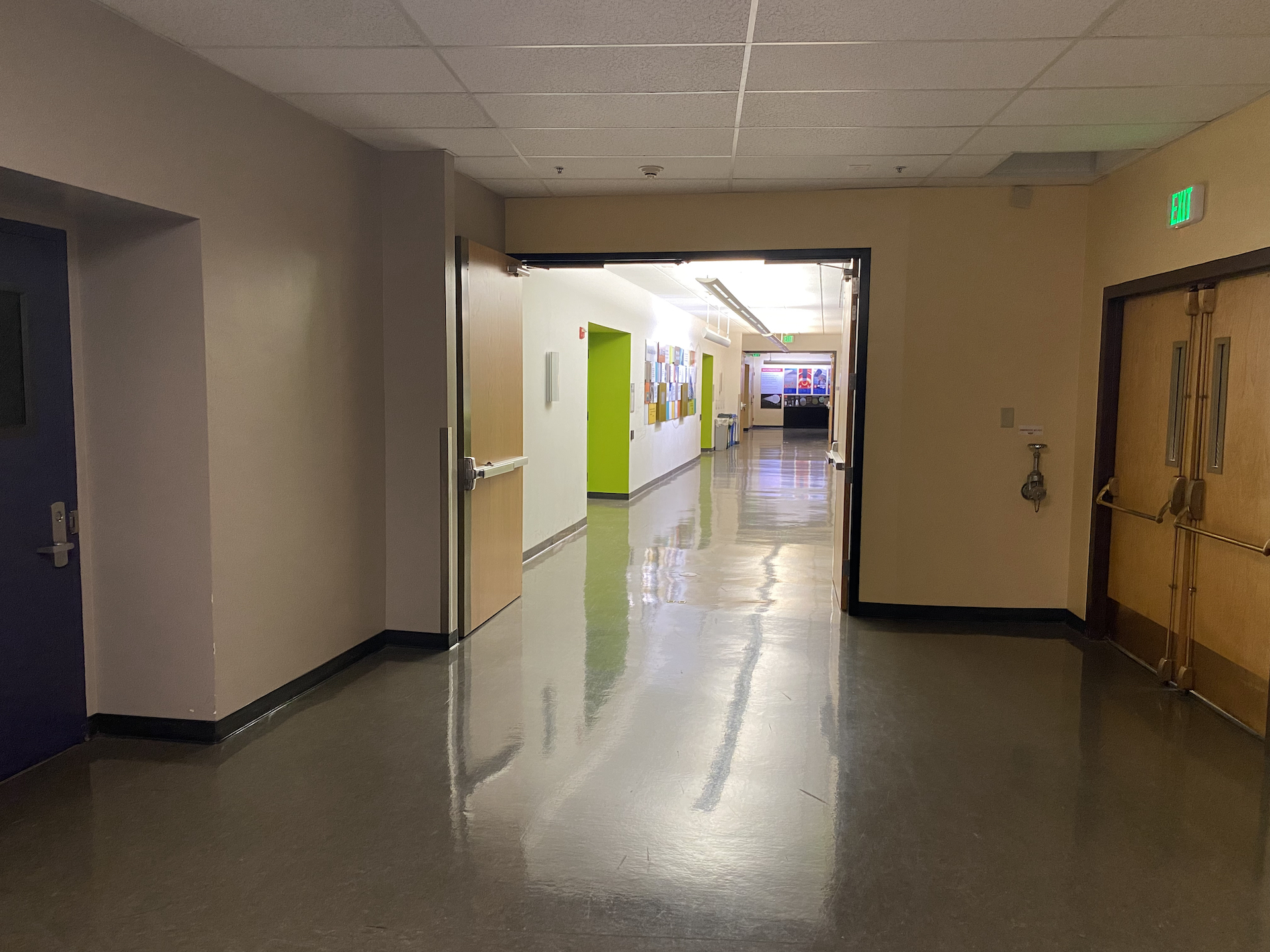
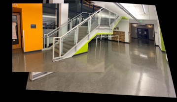
Cory Stairs

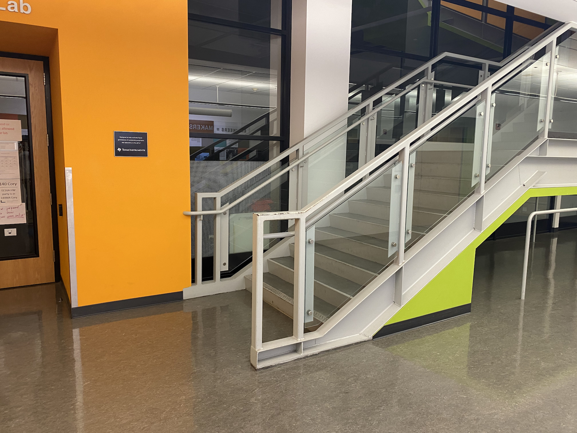
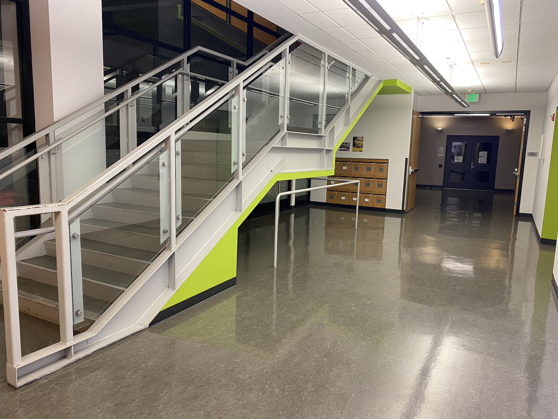
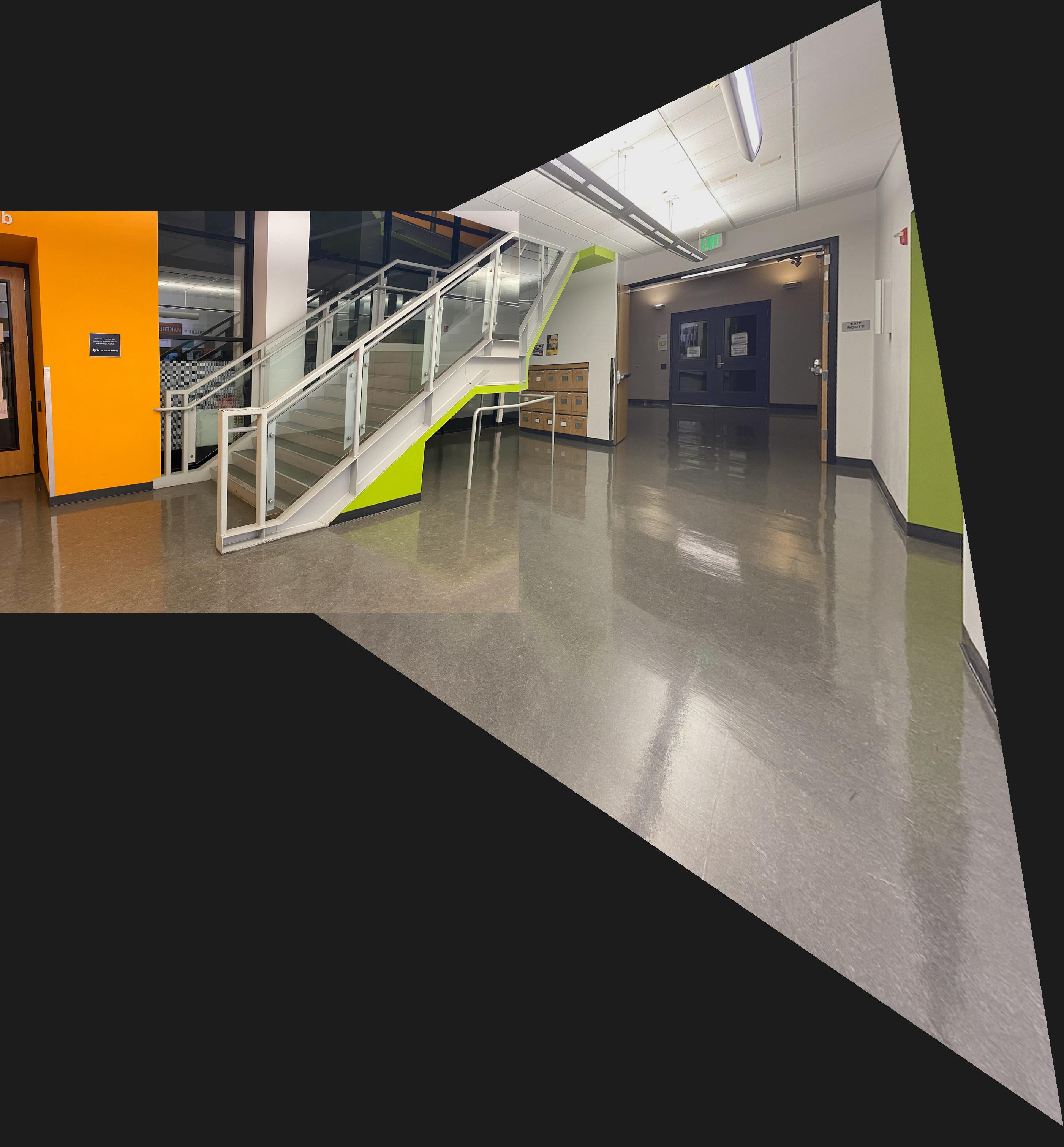
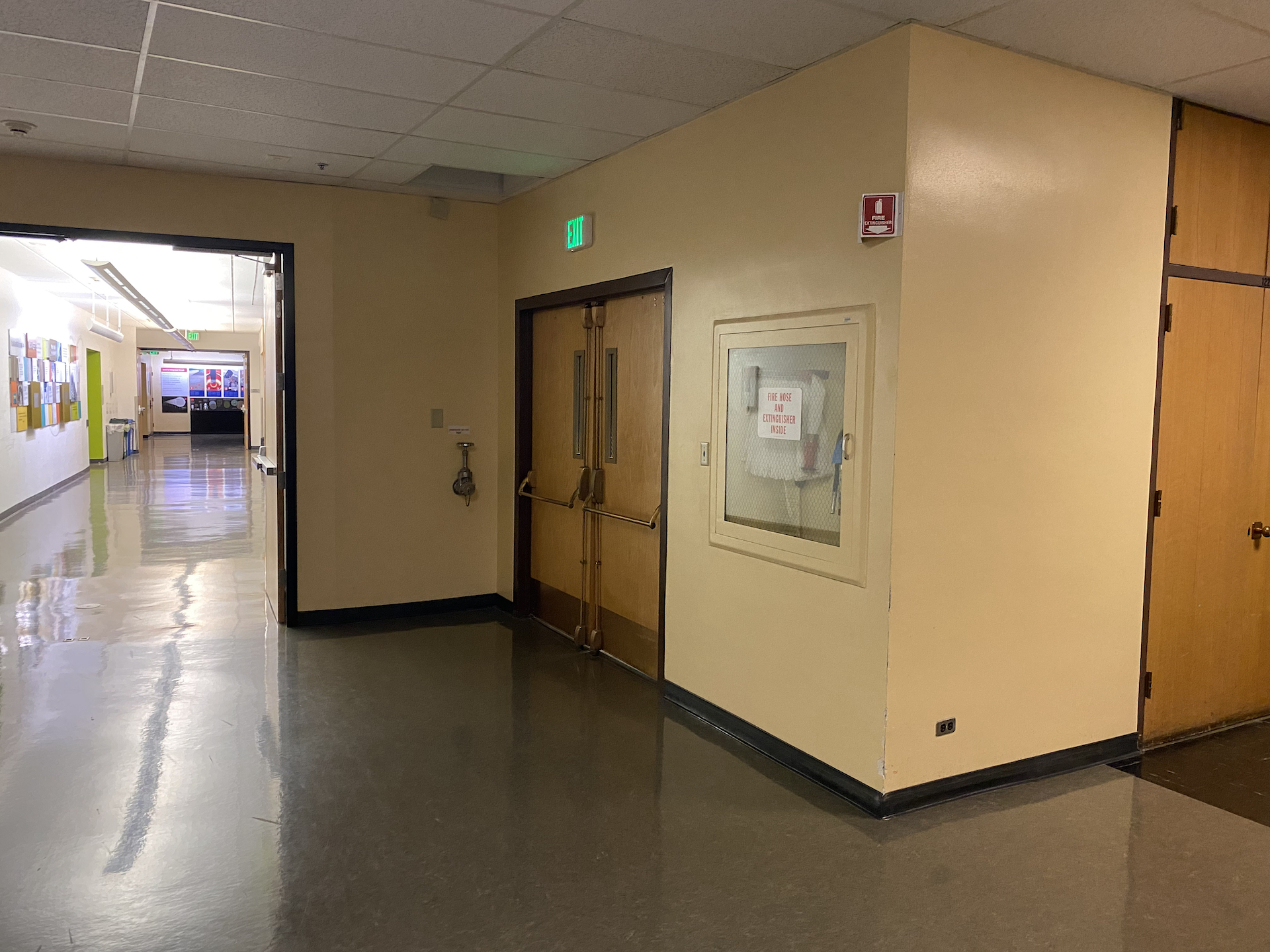
Cory Hallway

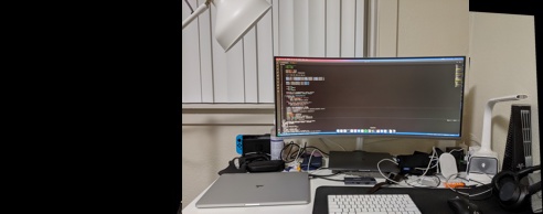
Desk

Part 1 Conclusion

In this part, the coolest thing I learned is how to project an image to a different perspective. It was very fascinating to see a top-down perspective on images, and the details it reveals about images that would not be obvious from the original image. It was interesting to me to see these details hidden in an image, and extracting this information was satisfying.

Part 2: Feature Matching for Autostitching

Harris Interest Point Detector

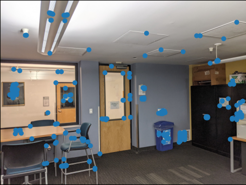
The Harris interest point detector is used to extract features from our images. This allows us to then identify the same features from different images. Here is an example of the features that we were able to extract with this algorithm:

Adaptive Non-Maximal suppression

Out of the box, the algorithm works relatively well. However, there are redundant corner points, and clusters of points. In order to achieve a better homography (and therefore a better stitching), we use adaptive non-maximal suppression to limit clusters, and spread out our points. Here is what the result of running this suppression looks like:

Feature Descriptor Extraction

After getting the coordinates of each feature, we need to be able to match the same features in different images. We accomplish this by sampling 40x40 clusters centered around each feature point, and scale down this cluster to be an 8x8 image. We then bias and gain normalize this feature descriptor to ensure that these features are invariant to differences in intensity. Here is an example of a random feature descriptor:

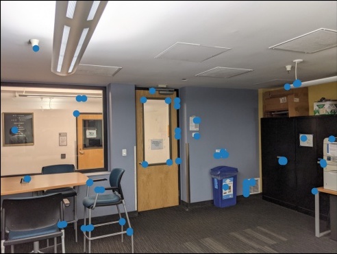
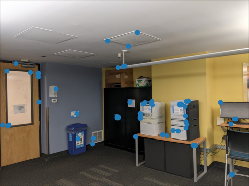
Feature Matching

Keeping Only Relevant Feature Descriptors

With all of these preperations in place, we can now actually match features, and stitch them together. First, we use the feature descriptors we created. We first compare all the feature descriptors of one image, and compare it to all of the feature descriptors of the other image. This comparison is done by finding the sum of square distances (SSD) between any two feature descriptors. We then pair images with the smallest SSD with each other, and verify that both feature descriptors in any pair have the lowest SSD with each other. We then keep all feature descriptors that have an complementary pair with a SSD below a certain threshold (in our case, the threshold was 0.3). Here is the result after filtering out and matching feature points:

As we can see, the same features are marked in the two different images.

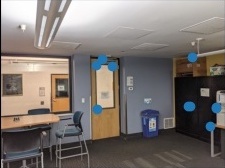
RANSAC

We use a random sample consensus (RANSAC) algorithm in order to find the best four corresponding points to use for our homography. Our notion of best is determined by the homography that creates the largest set of inliers given all our feature points. We consider a feature point to be an inlier after a homography transformation if the transformed feature point is less than some distance (in our case, a Euclidean distance of 2 pixels) away from its corresponding point in the other image. Here is the result of running this process:

Creating the Mosaic

Finally, we use the best homography that we have found from the RANSAC algorithm to transform our images into the same plane. Here is the result:

Mosaic Results

Part 2 Conclusion

RANSAC was easily the coolest algorithm that I learned in this project. It shocked me to see how such a simple algorithm could be so effective and accurate, and this was even more surprising when considering that one of the fundamental aspects of RANSAC is randomness.