In this assignment, I took two or more photographs and created an image mosaic by registering, projective warping, resampling, and compositing them. Along the way, I learned how to compute homographies, and how to use them to warp images.
I went outside and took a bunch of photos. I was careful to make sure to take several photos from the same center of projection. I did this by rotating my phone about the camera as I took several photos of a scene. I also used the AE/AF lock on my iPhone to make sure the camera settings would not change as I took photos.
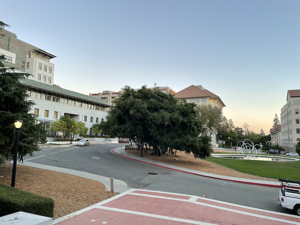
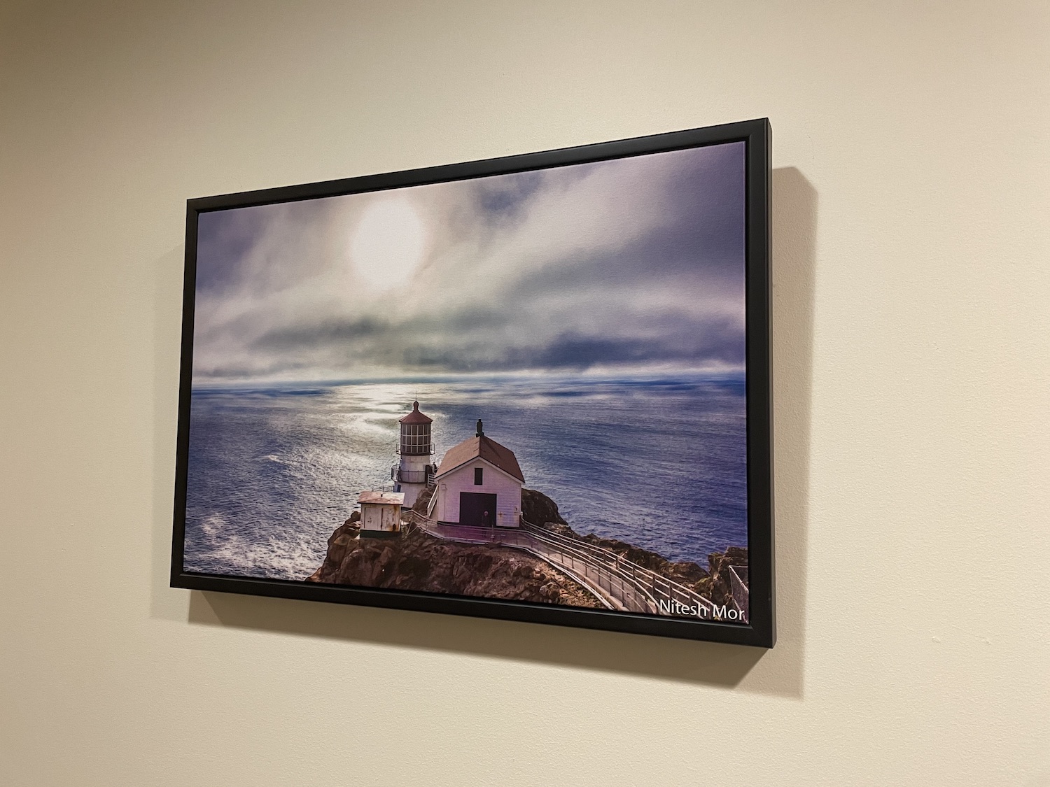
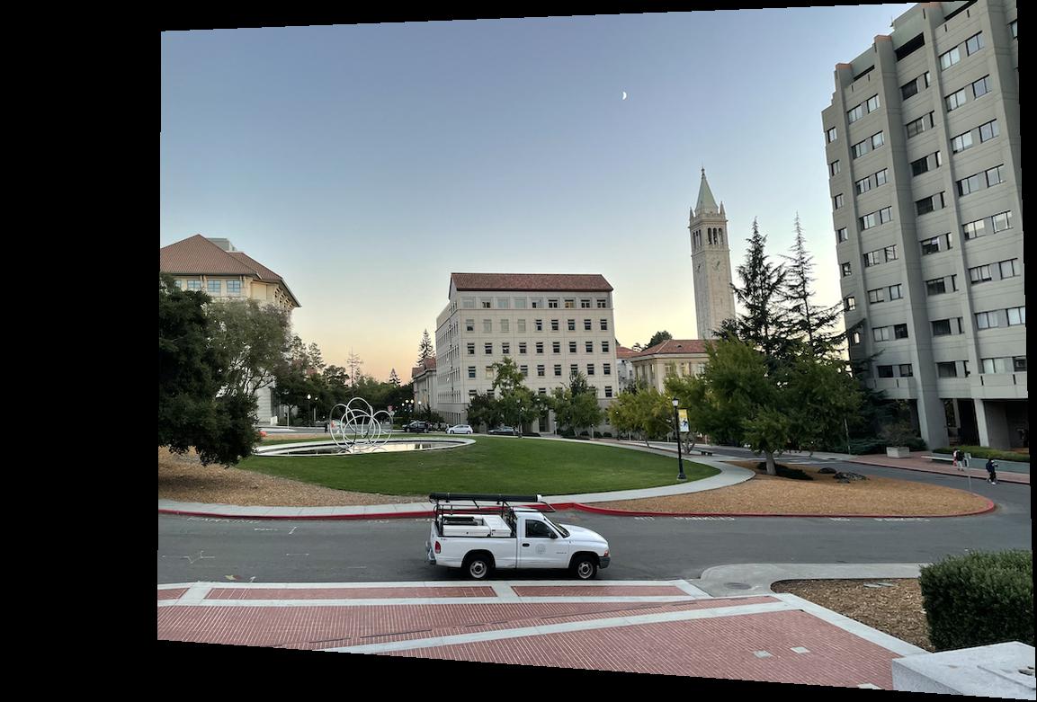
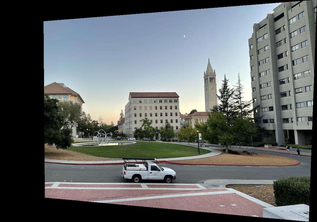
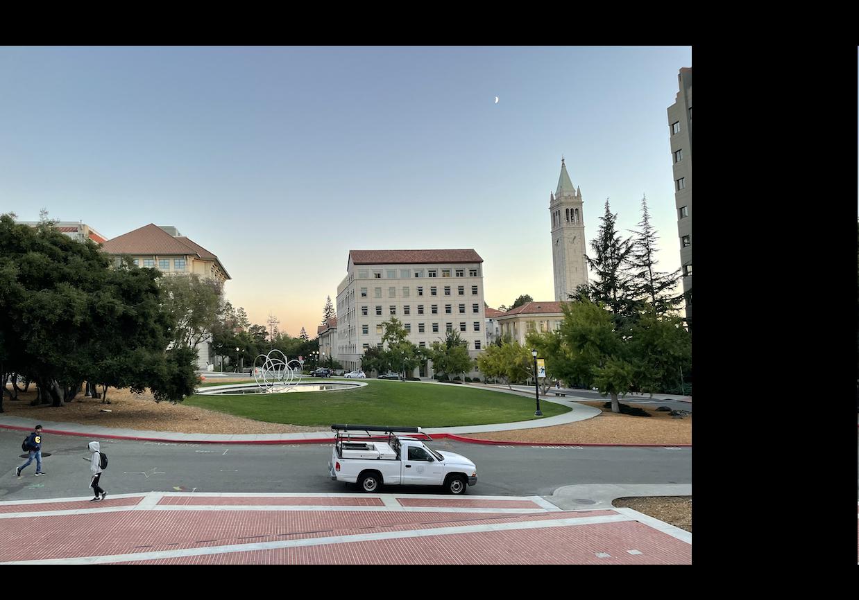
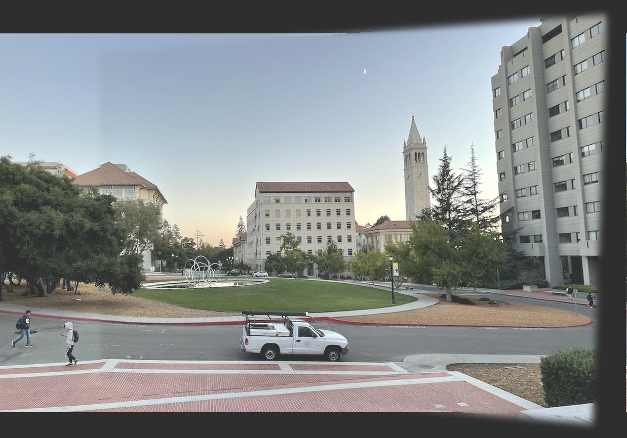
Some photos from Hearst Mining Circle
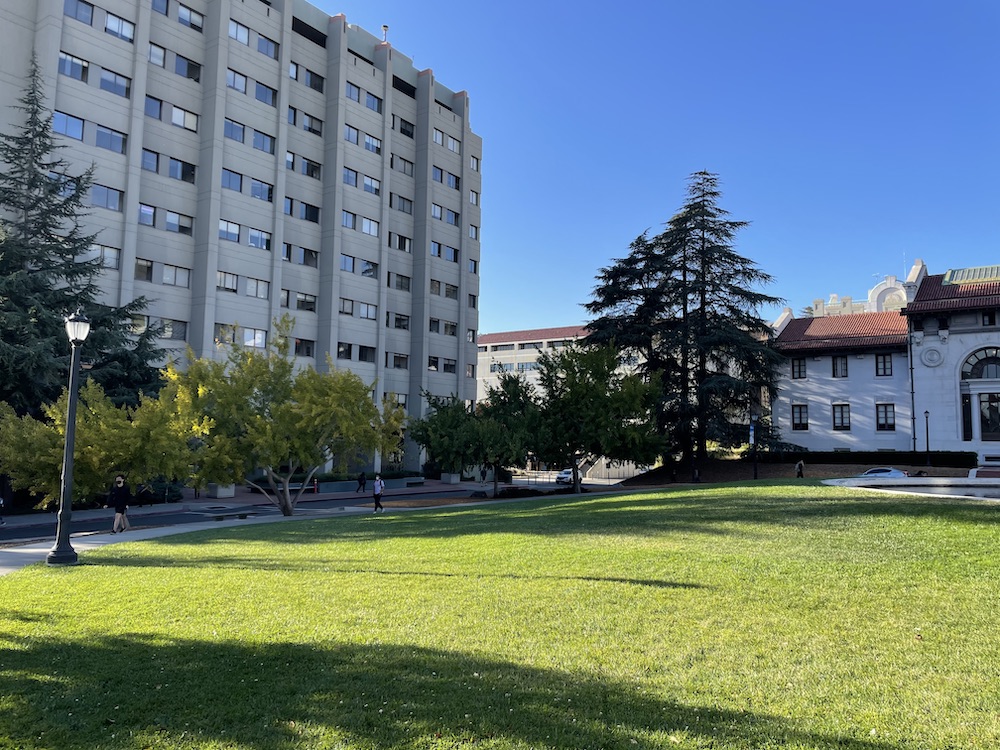
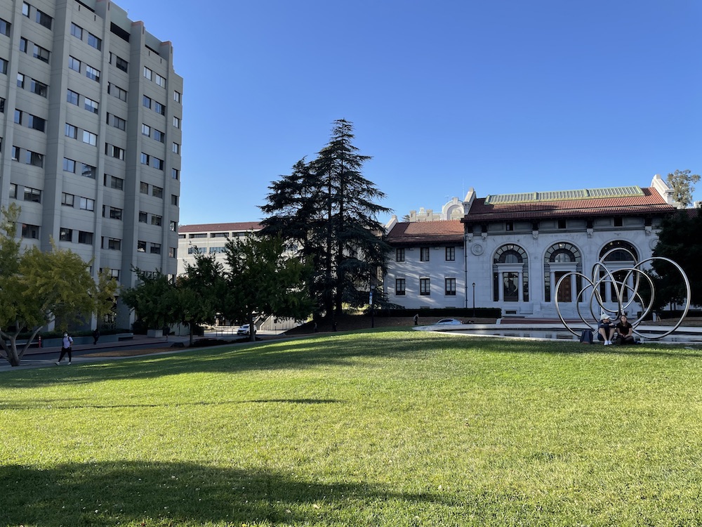
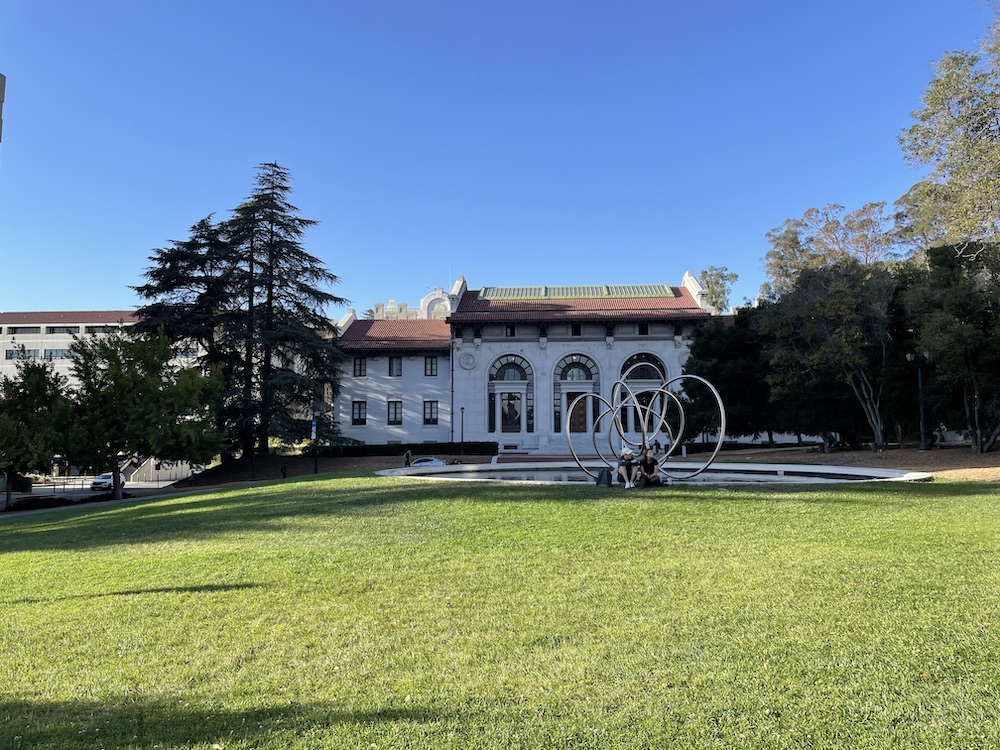
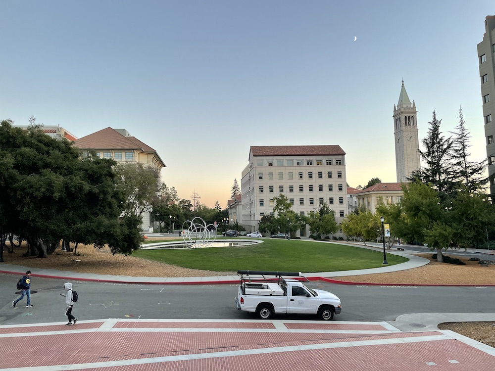
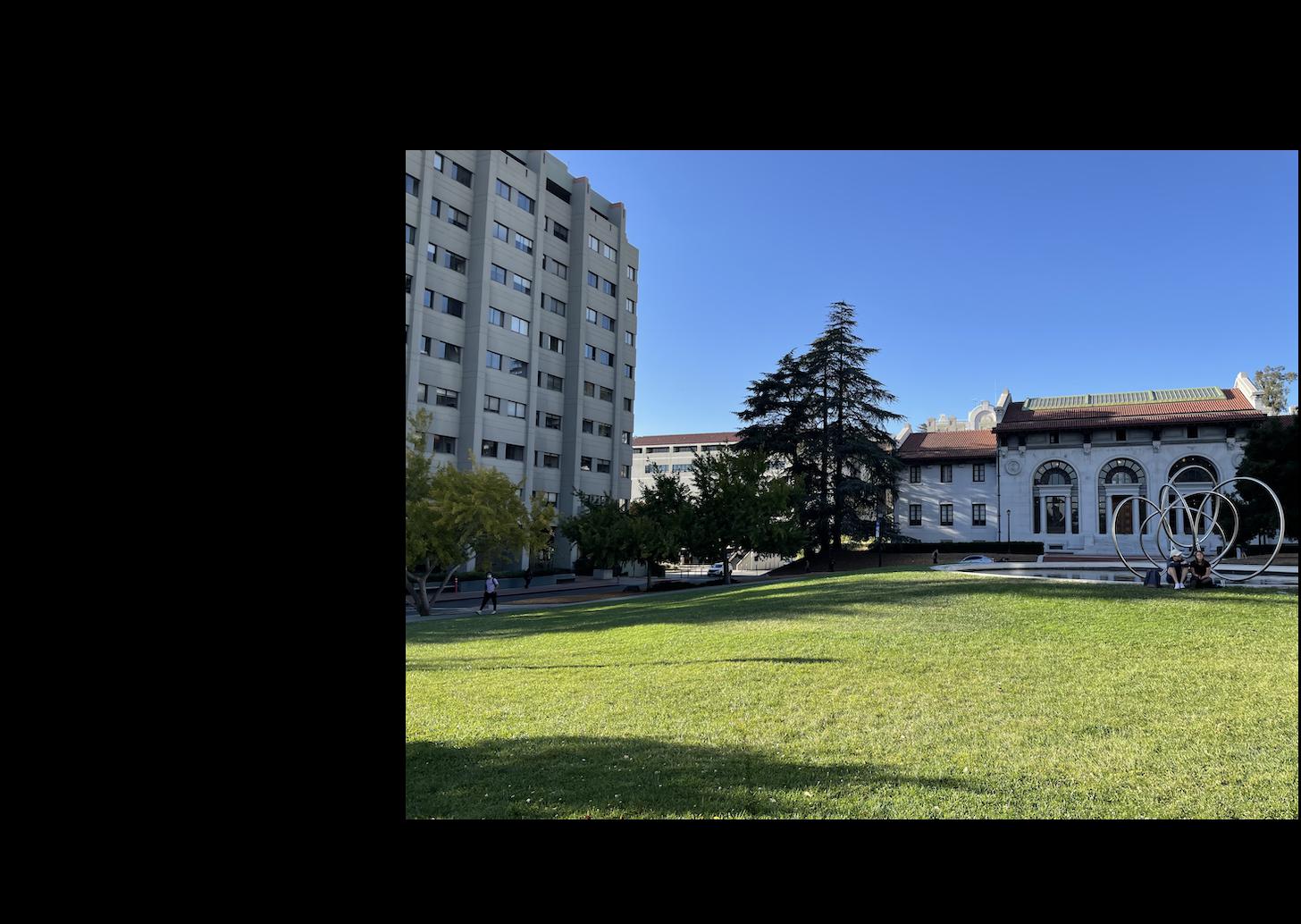
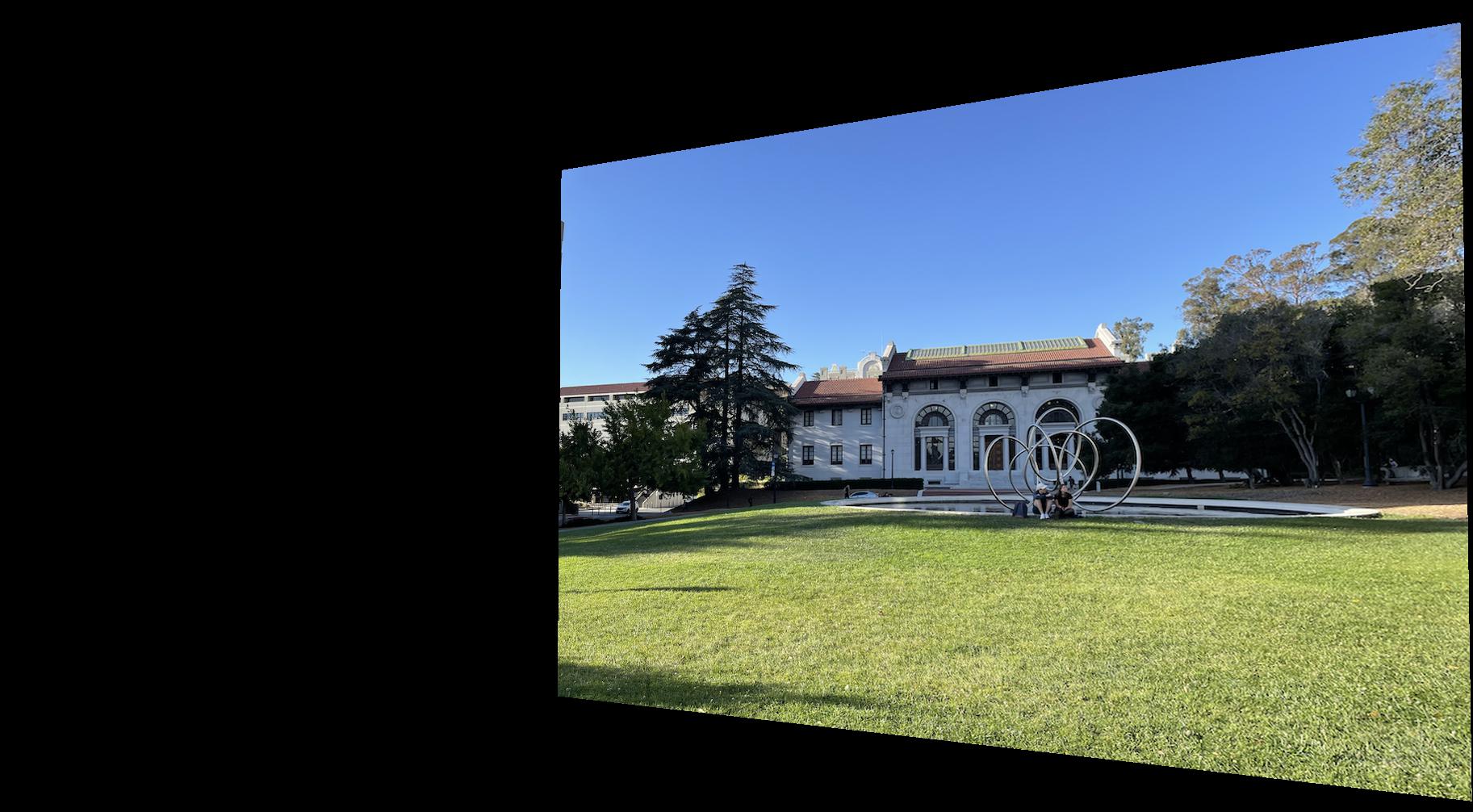
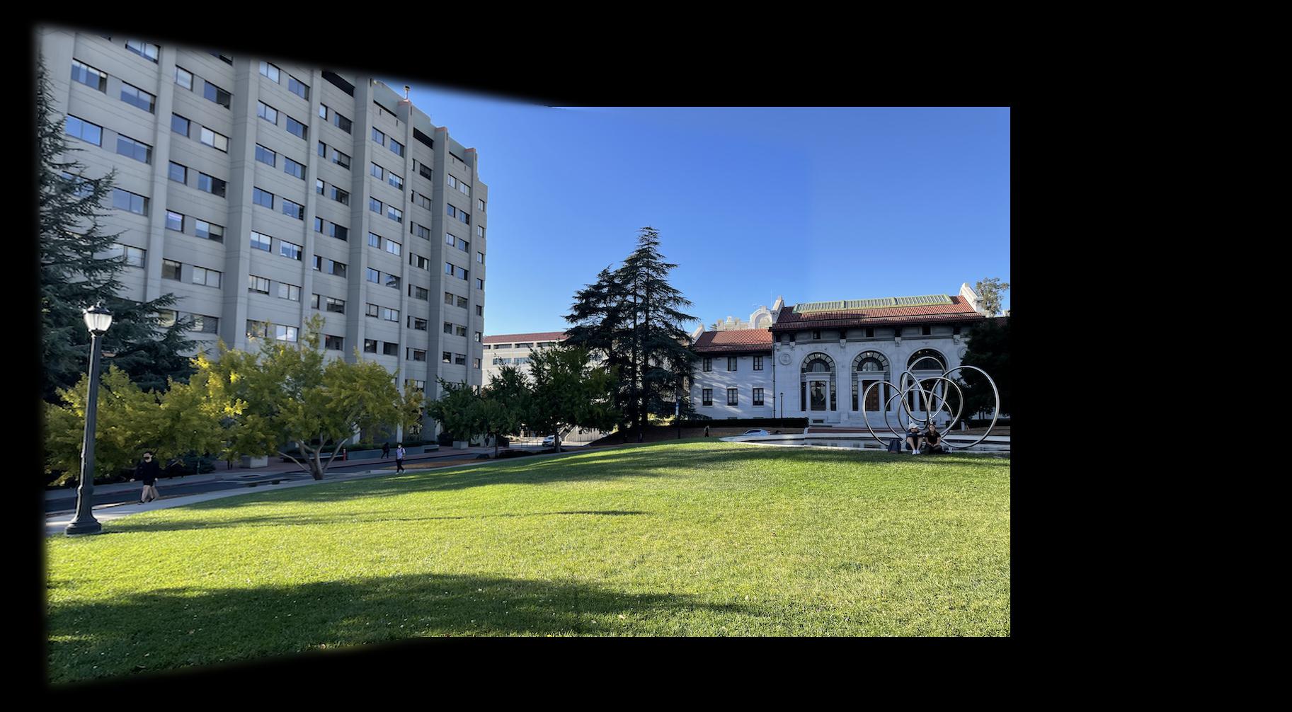
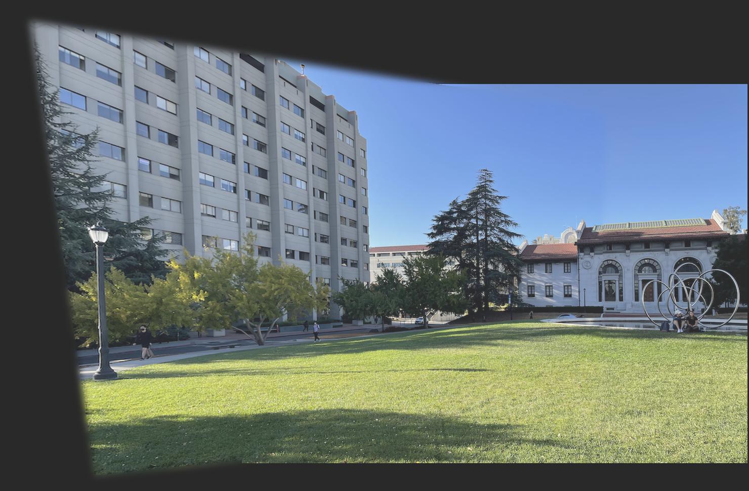
Some photos from taking from standing on the steps of Hearst Memorial Building

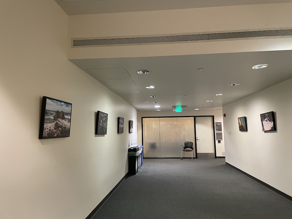
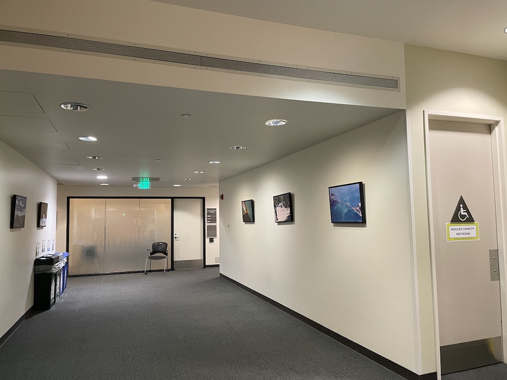
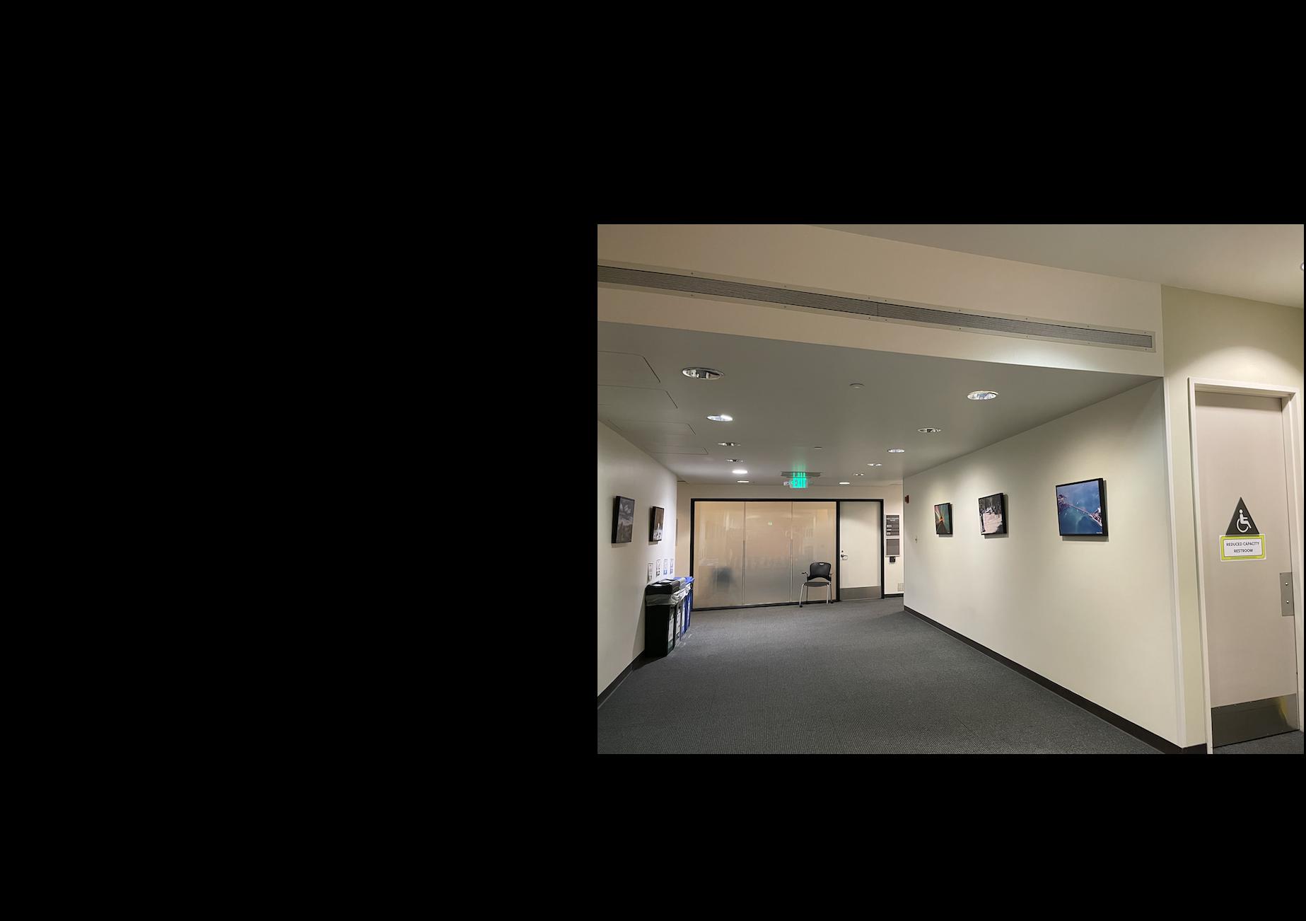
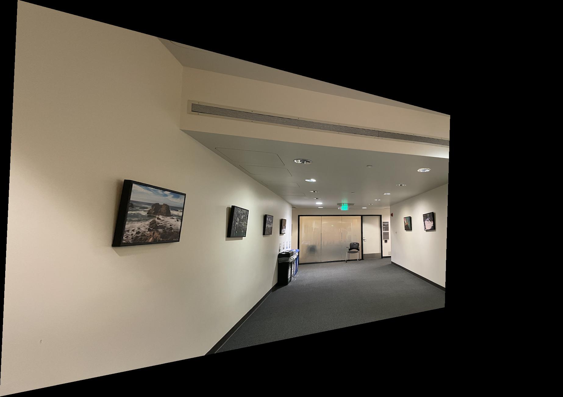
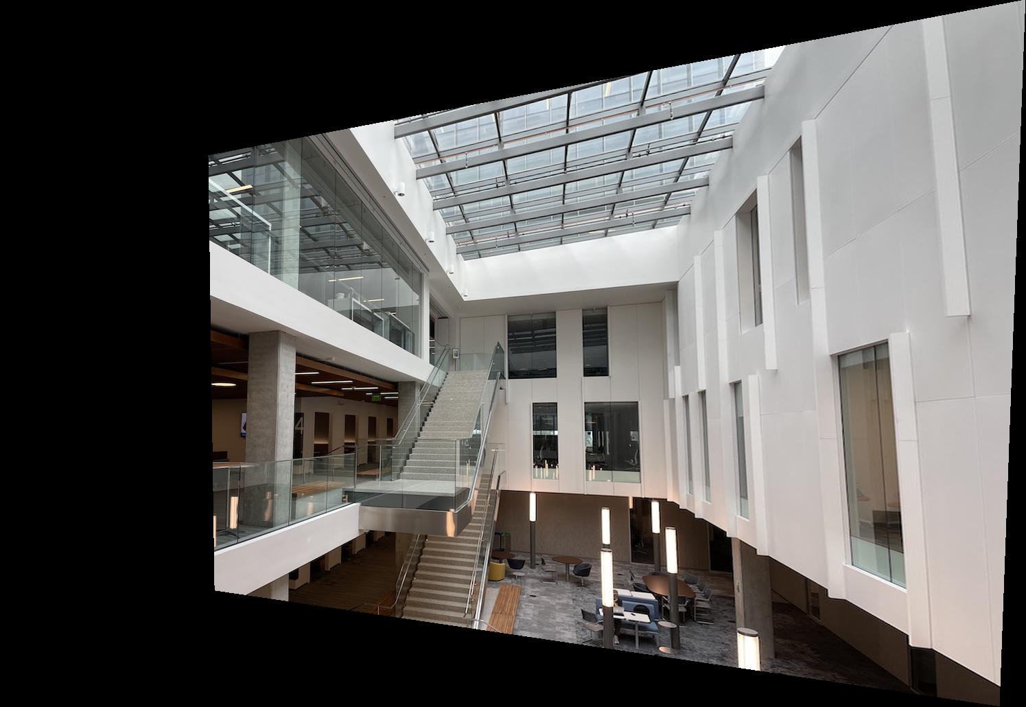
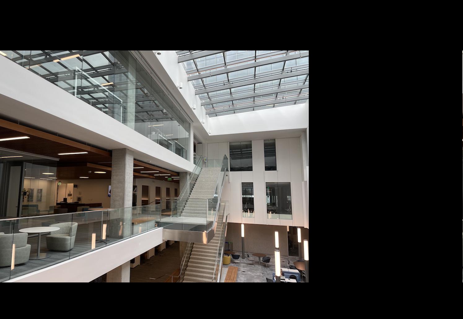
Some photos of Soda 5th floor
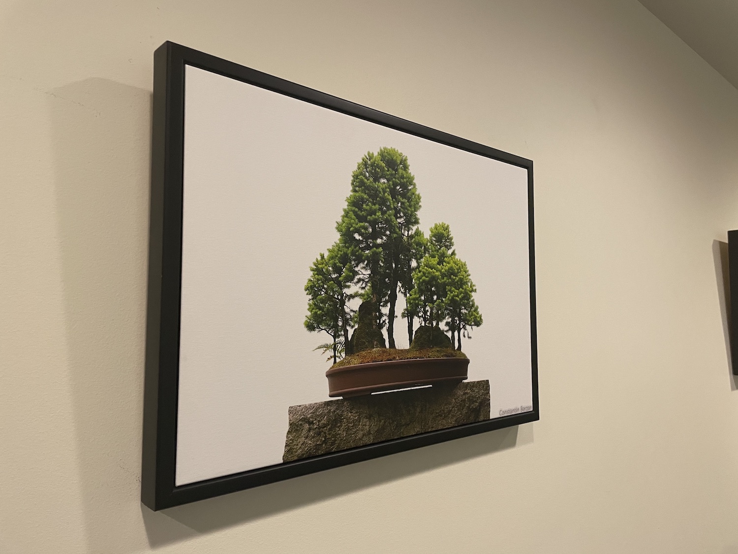
I also took some photos of rectangular shapes at an angle, so that I could rectify them later.
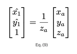
Homography lets us relate two cameras viewing the same planar surface. Both images are related by homography H as long as they are views of the same plane from a different angle. Let (x_1, y_1) be a point in the first image, and (xˆ_1, yˆ_1) be the corresponding point in the second image. Then, these points are related by the estimated homography H, as follows:
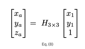
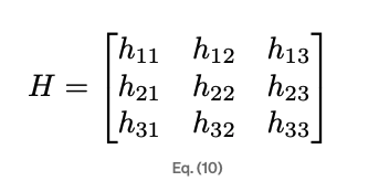
We can represent the homography matrix H as a 3x3 matrix with 8 degrees of freedom.
Since we have 8 degrees of freedom, we need at least 4 points to solve the system. However, in order to reduce error from selecting our points, we can overdetermine the system by selecting more points and then using Least Squares to solve for the constants that minimize our error. We rearrange our system of equations to get an matrix multiplication in terms of a vector containing all of our unknowns.
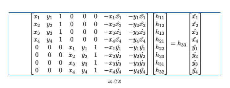
Instead of just using 4 points though, we use N points to get a matrix of 2N x 8. We then solve for this system by using np.linalg.lstsq(A,b) where A is our matrix and b is our vector of unknowns.
I then wrote a `warp_onto` method that took in an image to warp, the base image, and a homograph matrix H. Using that, I warped the corners of the first image to get the polygon of the warped image, and then used a inverse warp to fill the rest of it in. After that, I created a mask in the shape of the warped image (but slightly smaller so that I wouldn't get the weird black borders), and used a Laplacian pyramid to blend the two images together. See the next two parts for examples of this.
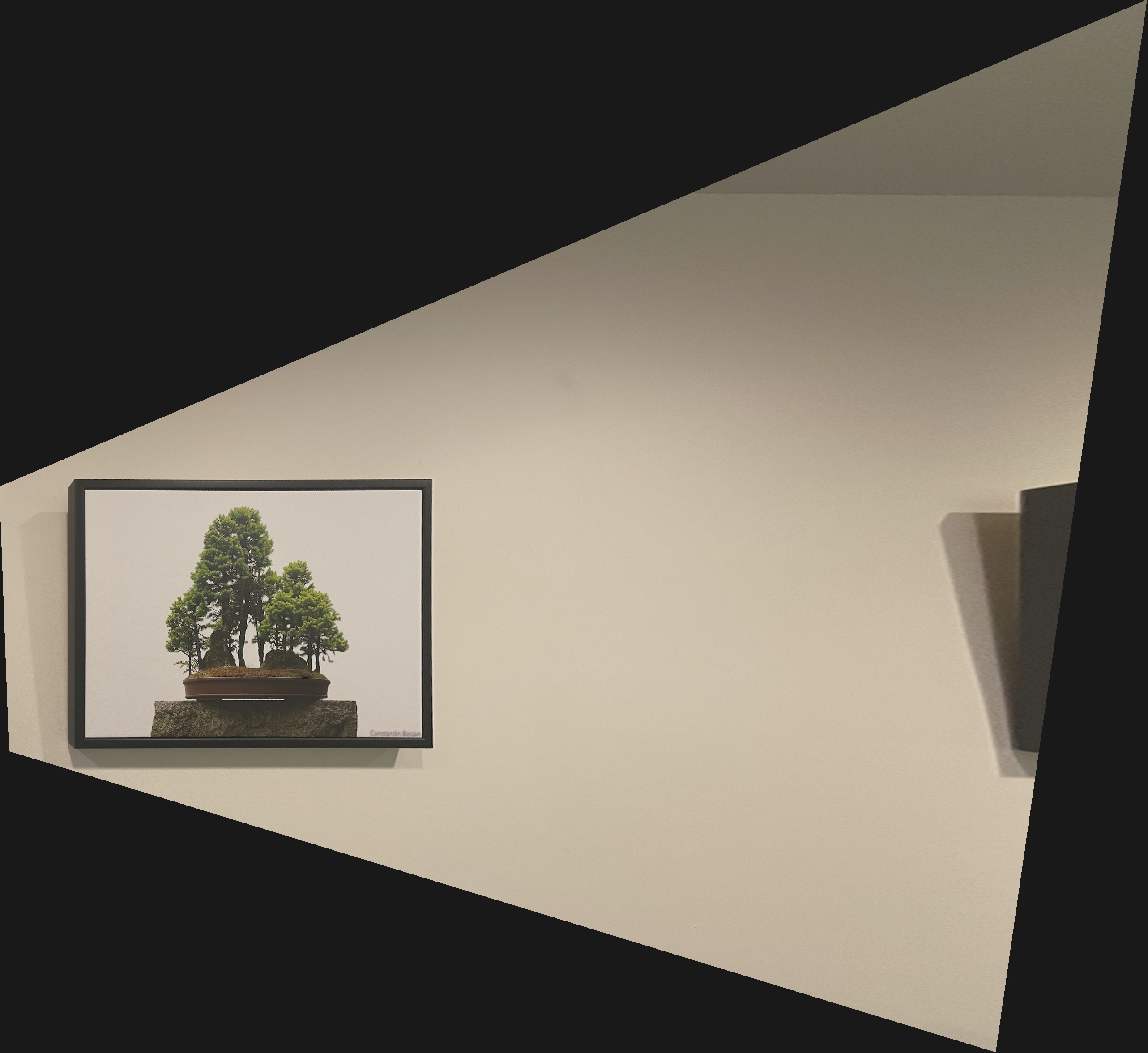
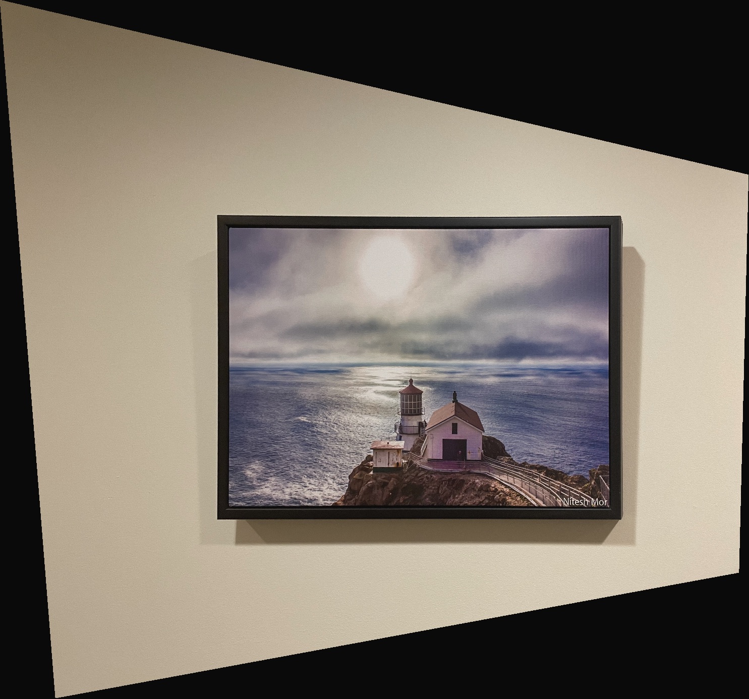
I took some images with some planar surfaces, and using my warping algorithm, warped them so that the plane is frontal parallel. I did this by simply defining a rectangle with some user-defined dimensions, and computing the homograph between points I selected, and the rectangle.
Here are some rectifications of photos on the wall of the 5th floor of Soda. Before on the left, after on the right.
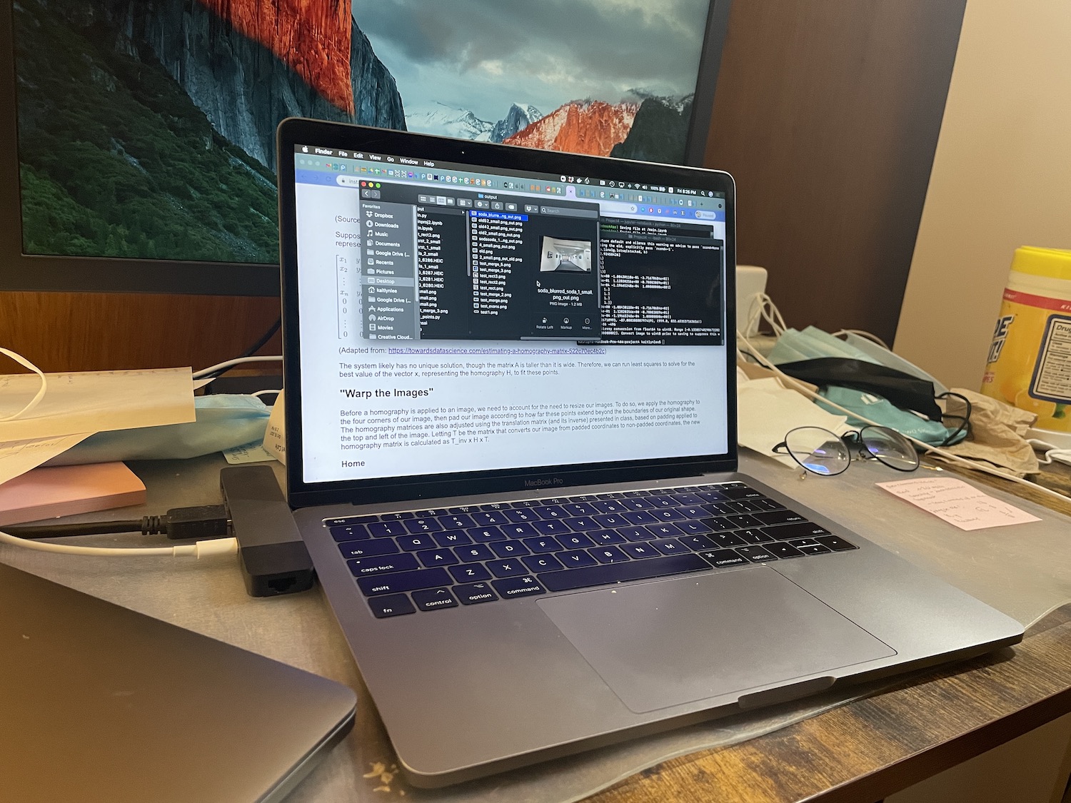
Here are some rectifications of my laptop screen.
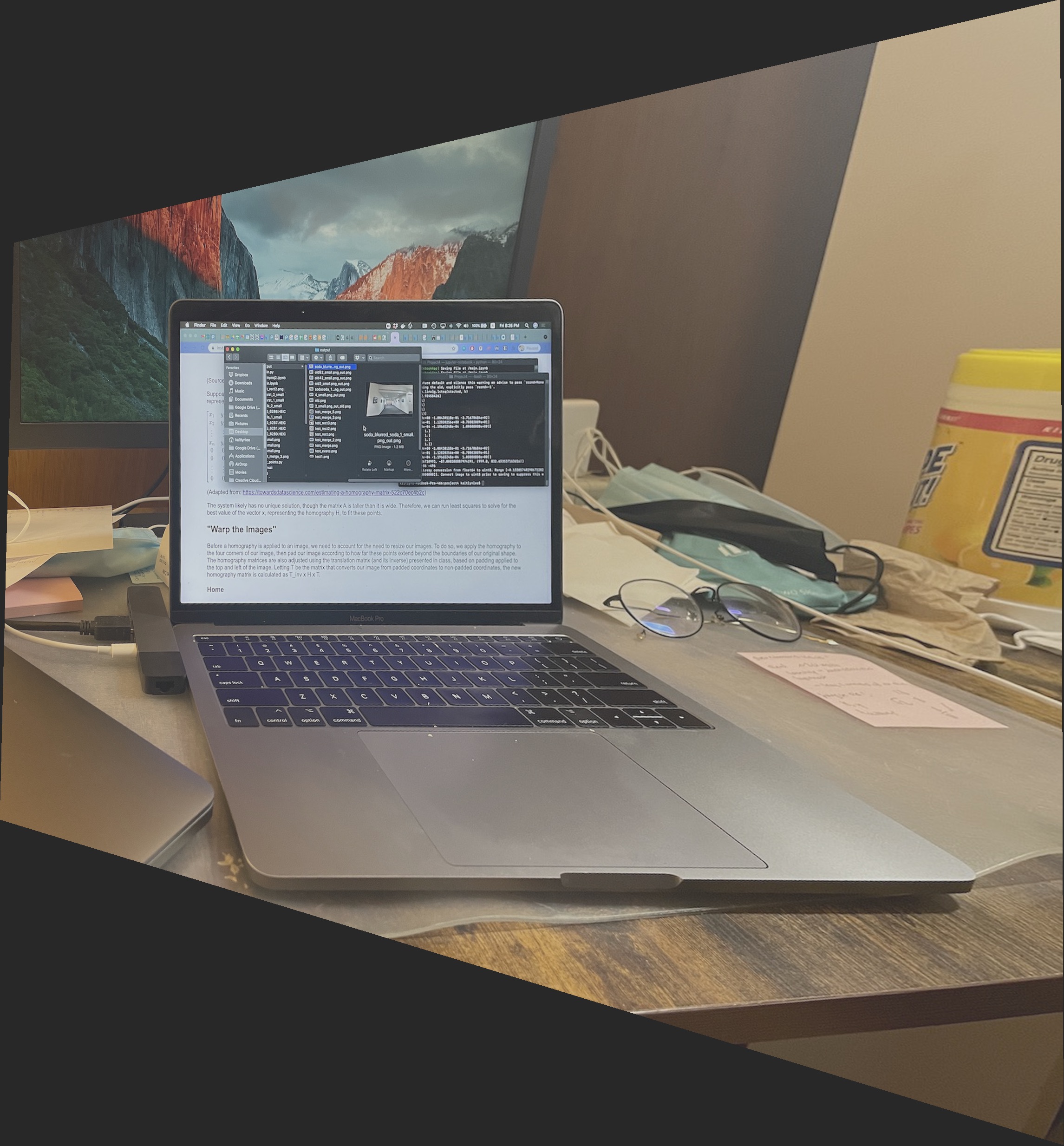
I also tried rectifying my laptop keyboard. However, something seems to have gone wrong. Perhaps the transformation was too drastic :hmm:
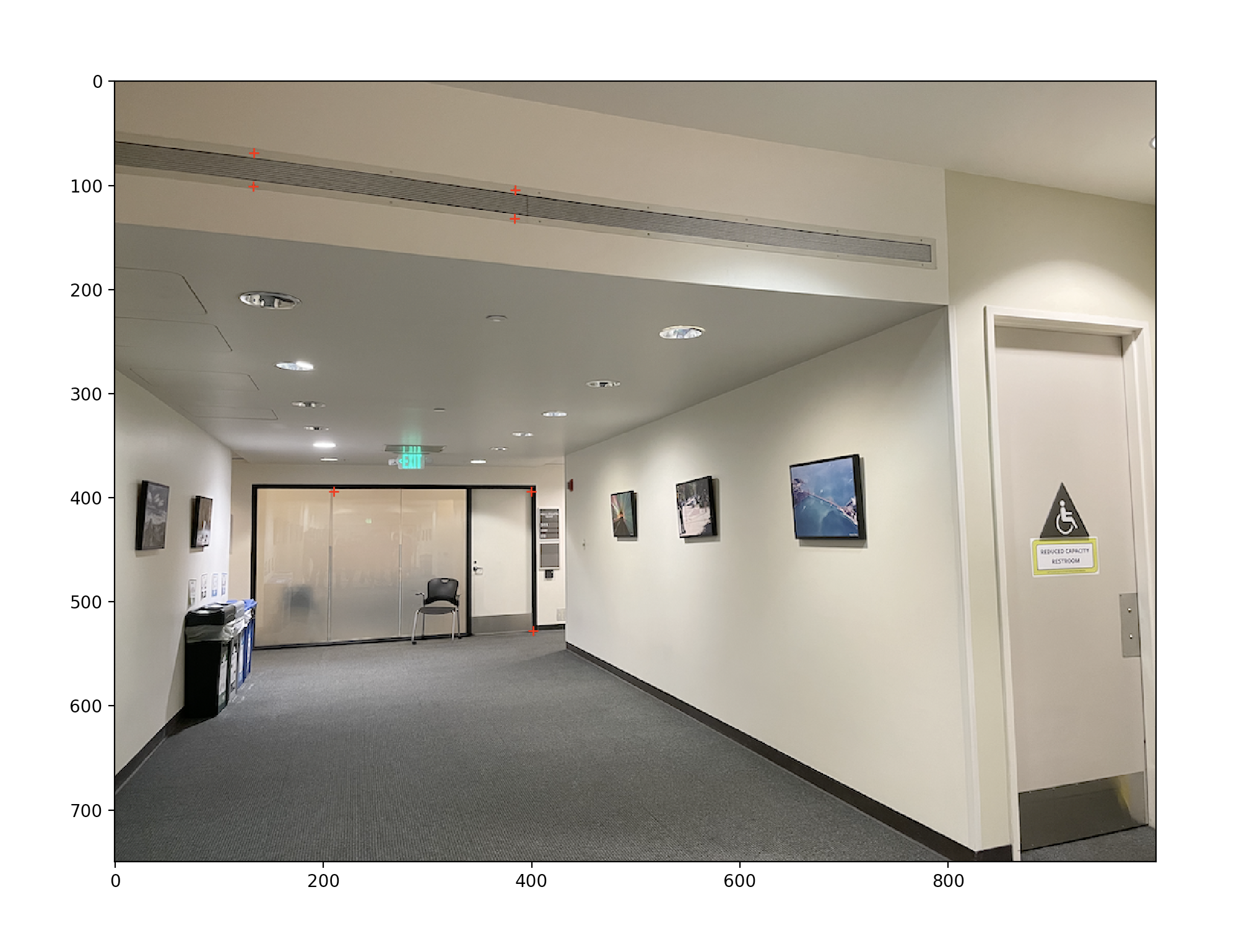
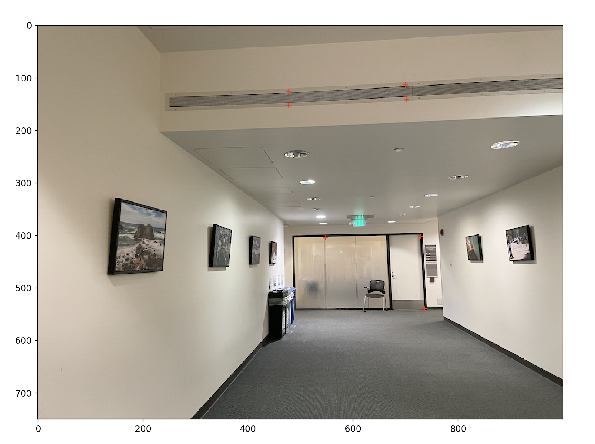
I wrote a script that would take in image names, prompt the user to pick the correspondence points on the image, and then morph the images together. It starts with the first image as the plane, and warps all other images onto it. Here are some examples of what my process looked like. Note that I used 8 points to define the correspondence, but there are only 7 in the photos due to me having to screenshot before picking the last point (lest the program continue running).
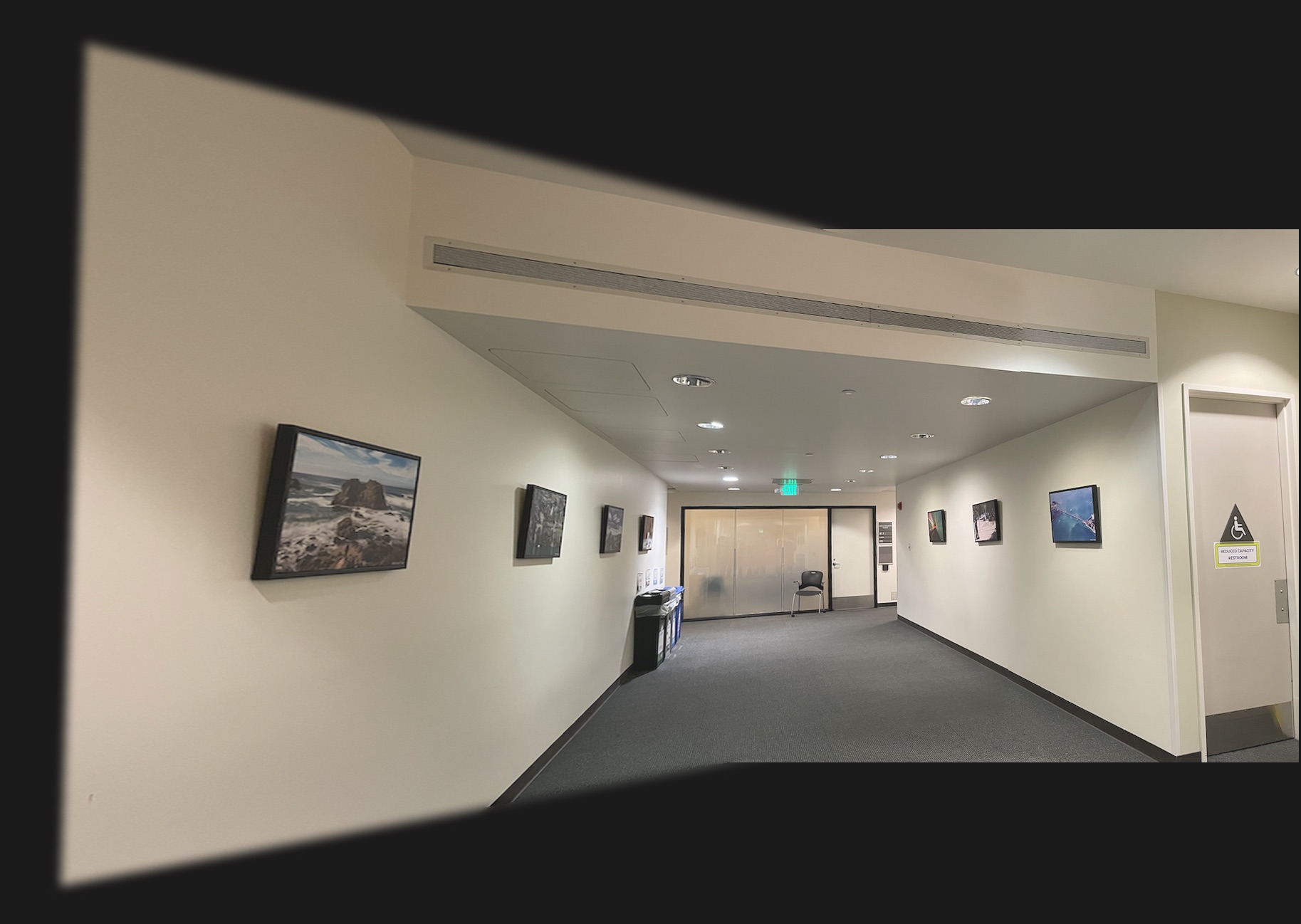
I also blended the images using a Laplacian pyramid, hence the blurry edges.
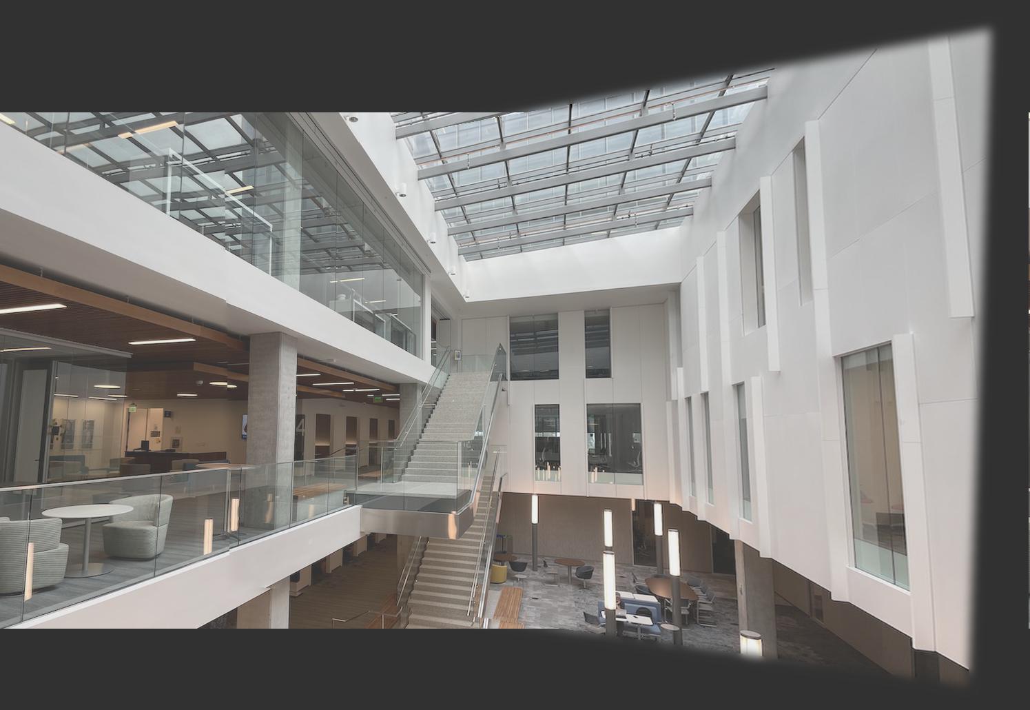
Here are the photos of Soda's 5th floor blended together. I first picked some points on both images. This photo had lots of nice rectangular images, but it was hard to find points that would line up the wall nicely.
Here are what the images looked like before merging.
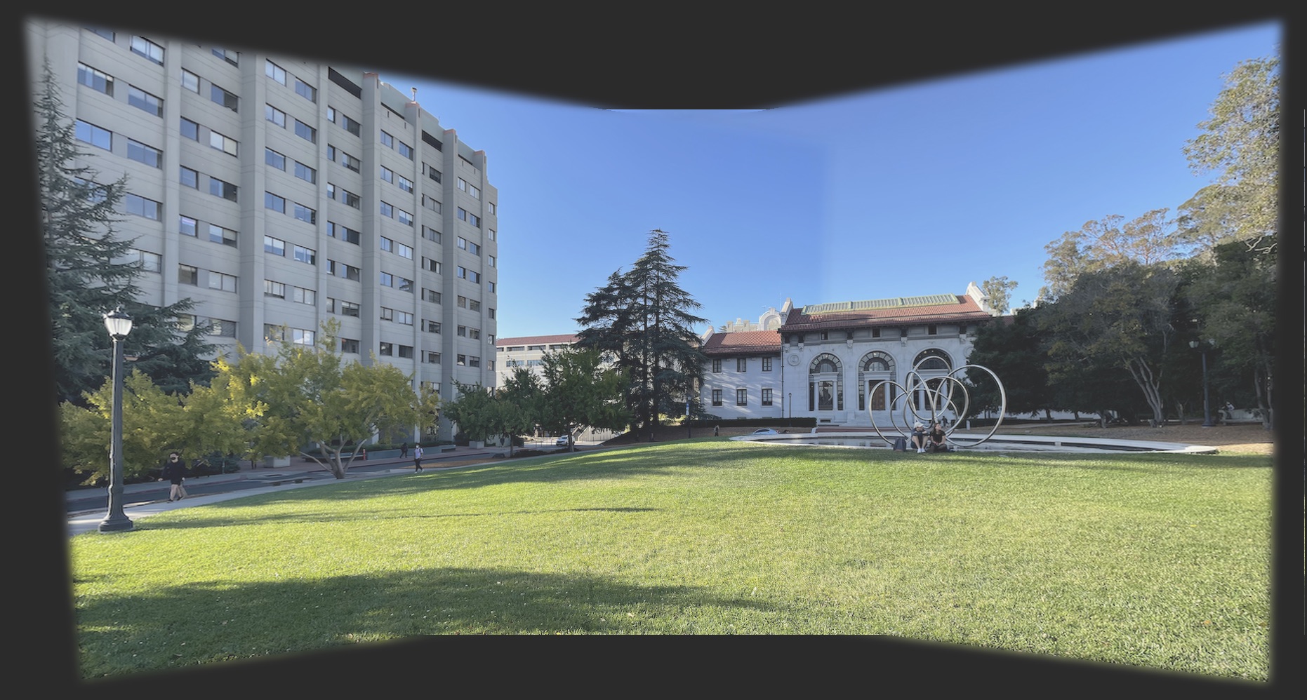
Here are the photos of taken of Evans and Hearst Mining blended together. I merged together 3 images for this one.
Here was my 2-step point selection. One between the first 2 images, and one between the morphed image and the third image.
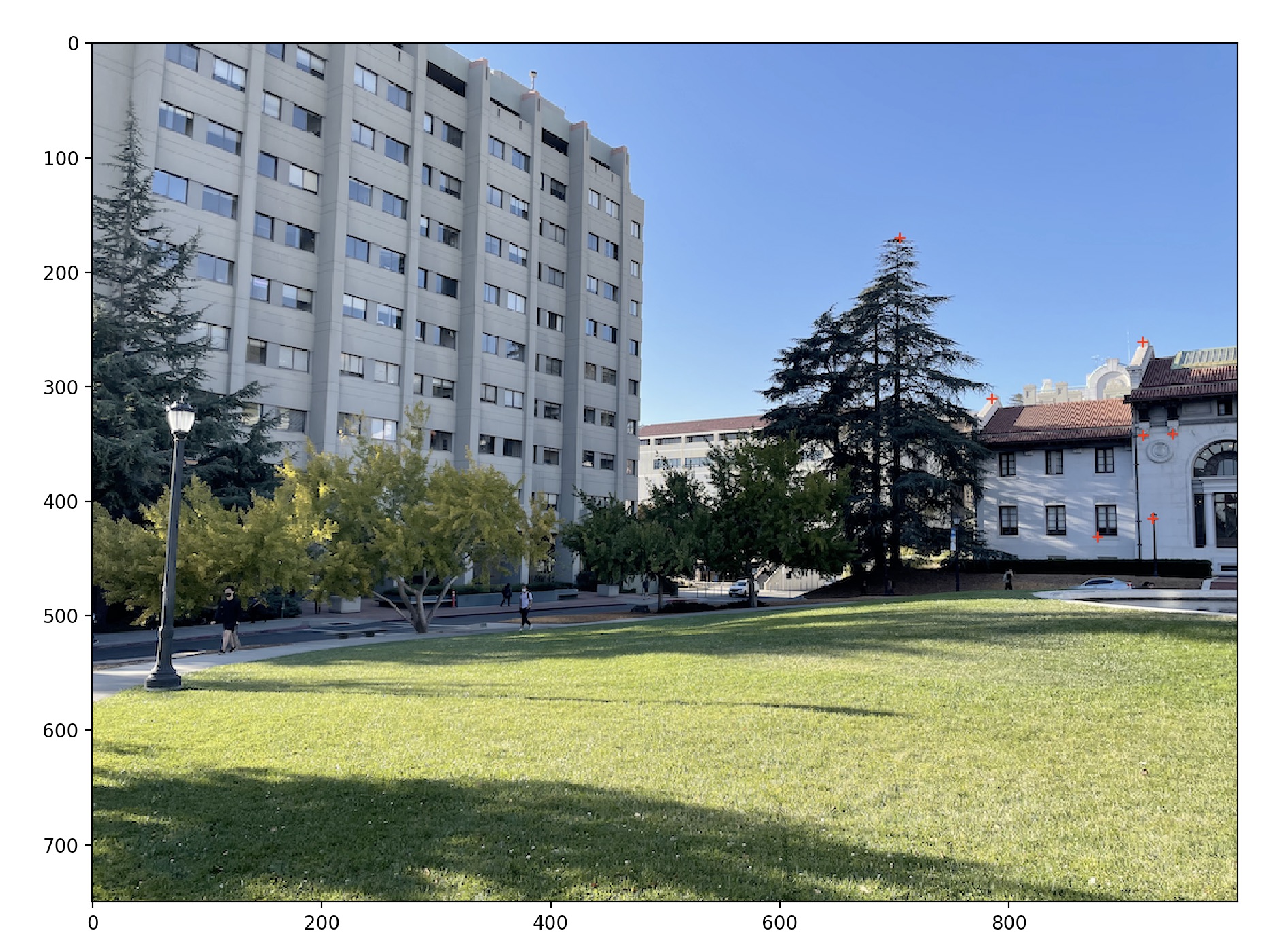
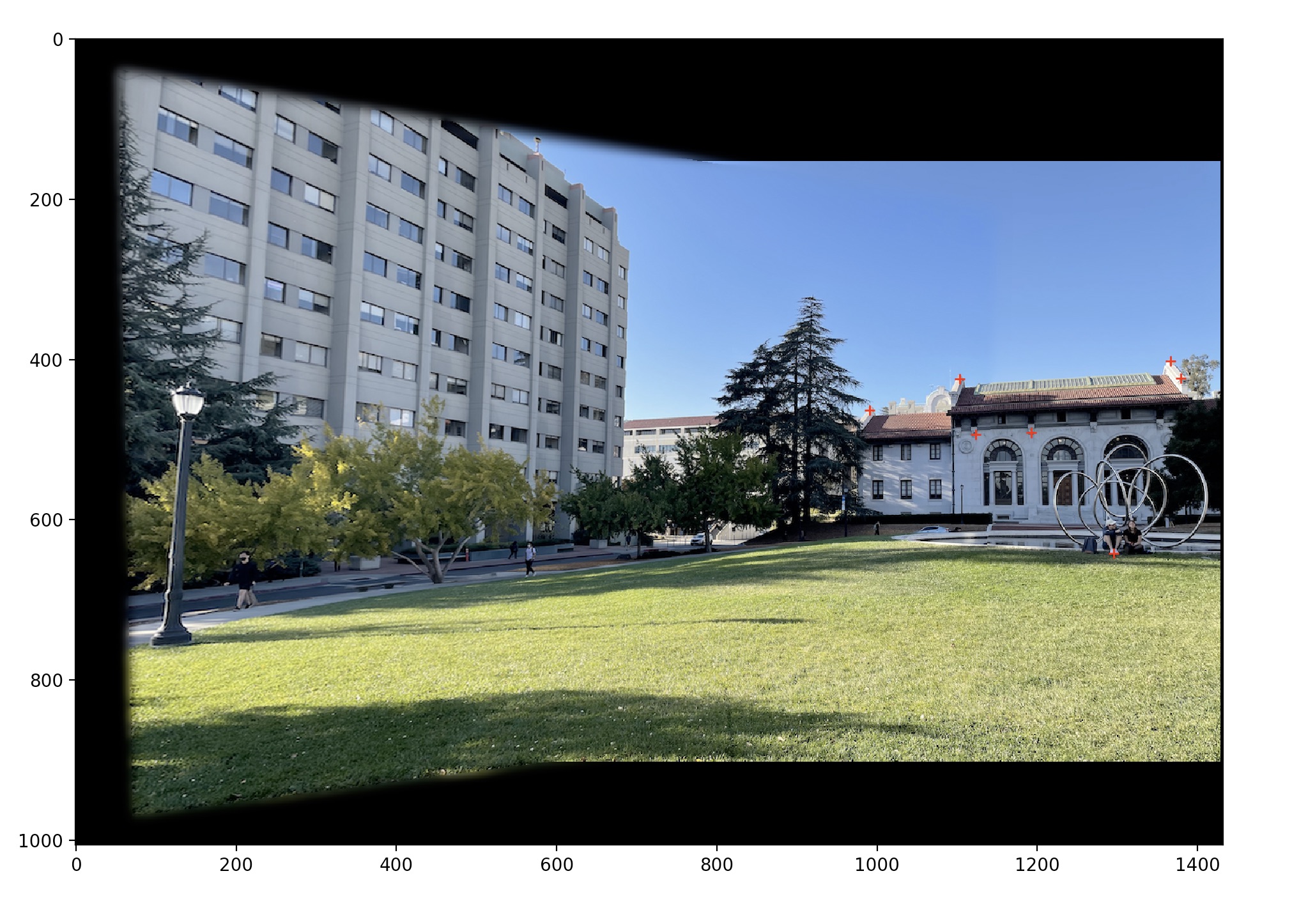
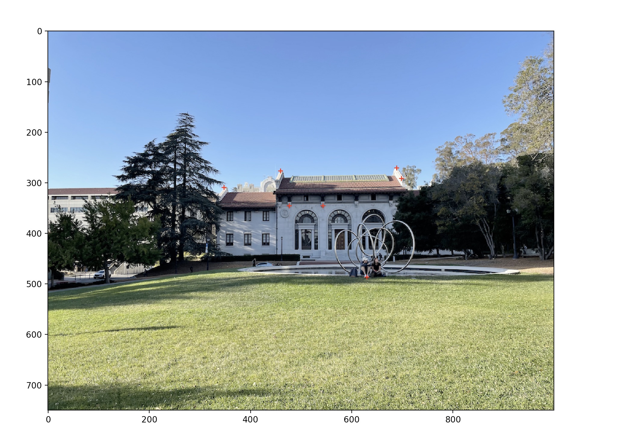
Here are what the images looked like before merging.
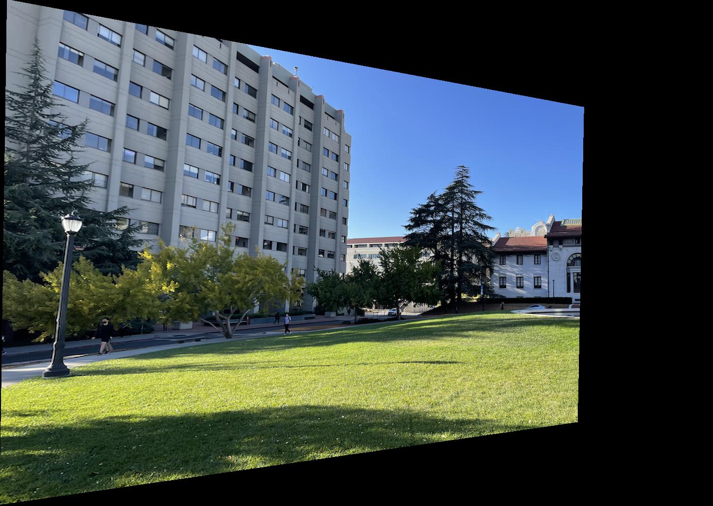
Here is the partial morph and then the full morph of all 3 images
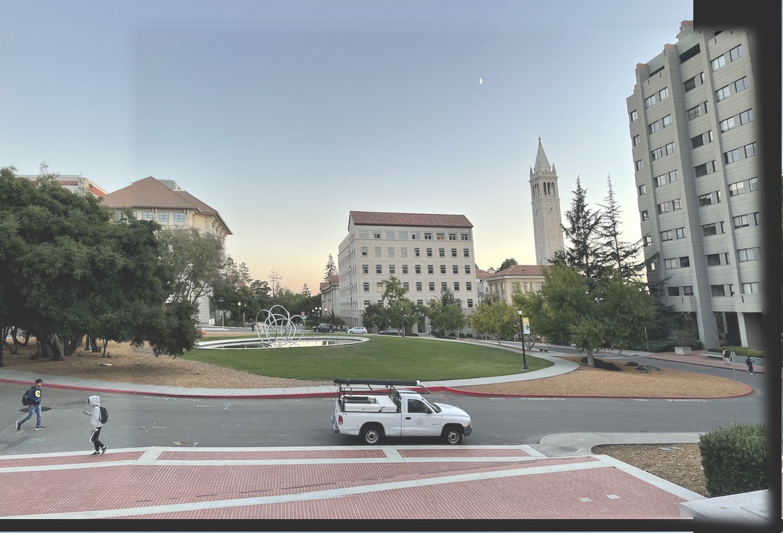
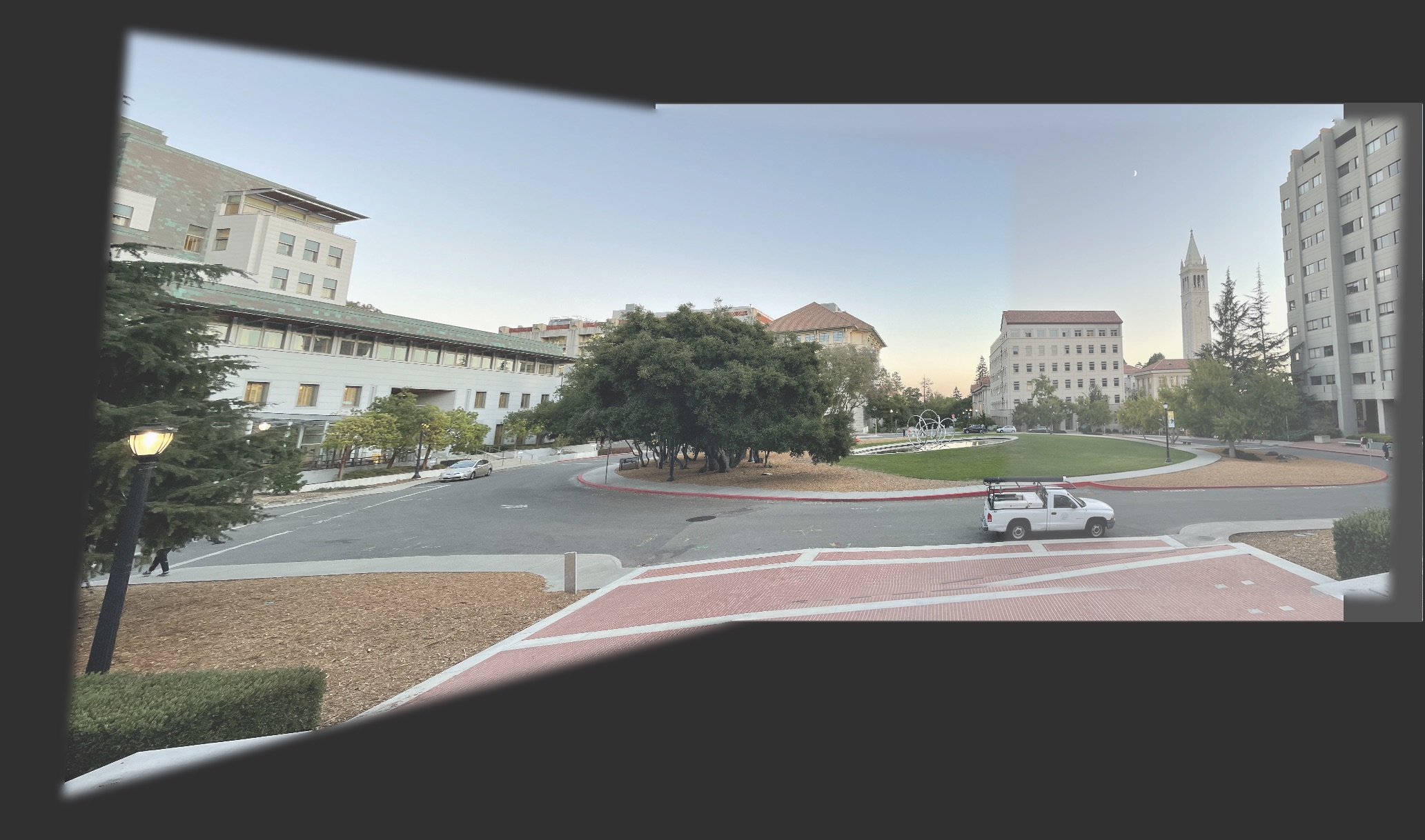
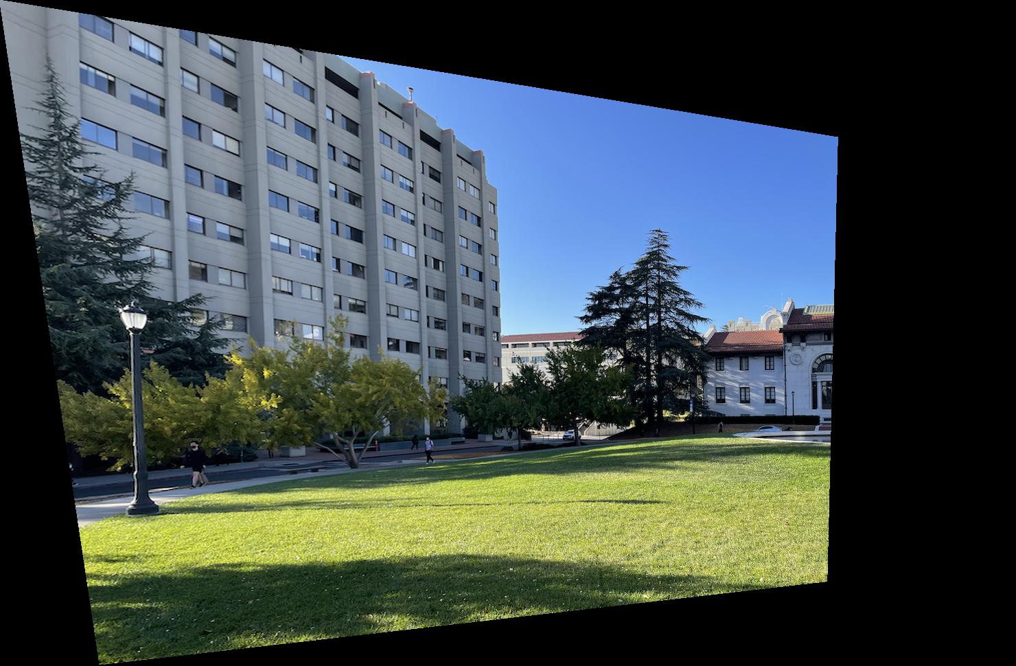
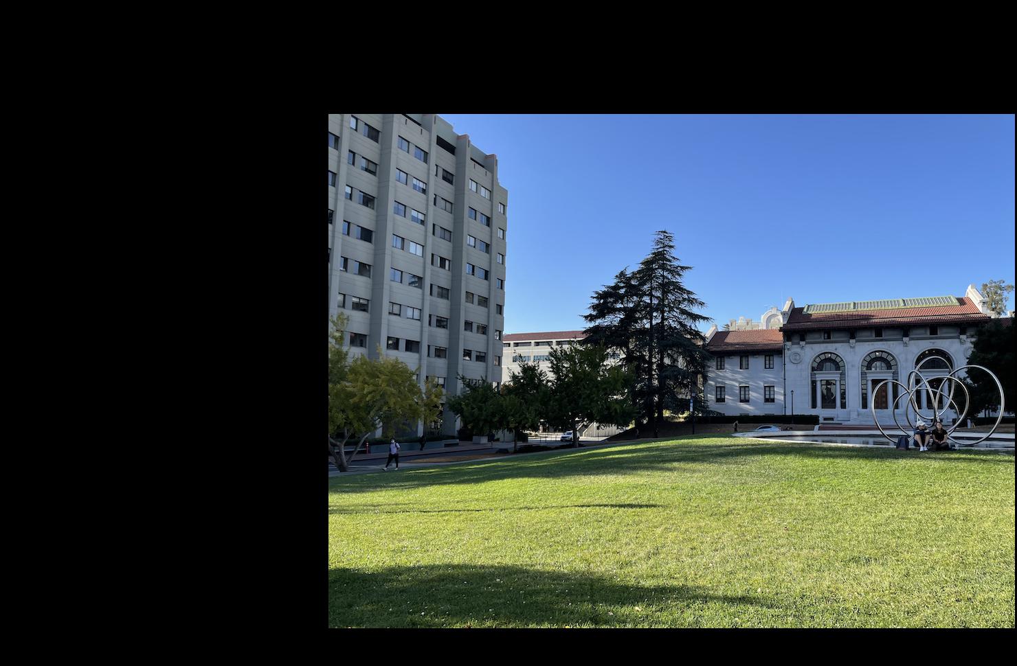
Here are the photos of taken of the other side of Hearst Mining Circle. I merged together 3 images for this one as well.
Here are what the images looked like before merging. (since the middle image was the one we were warping too, it was just an the same image but translated to fit the other images' scale)

Here is the partial morph and then the full morph of all 3 images
I thought this part of the project was really cool! I had a lot of fun running around campus and taking photos. However, I learned that the points I choose have to be pretty precise. For some images, I reselected the points dozens of times before I found ones that lined up perfectly.
In this part of the assignment, I took two or more photographs from the previous part (along with some new photos) and wrote a method to automatically create a mosaic.
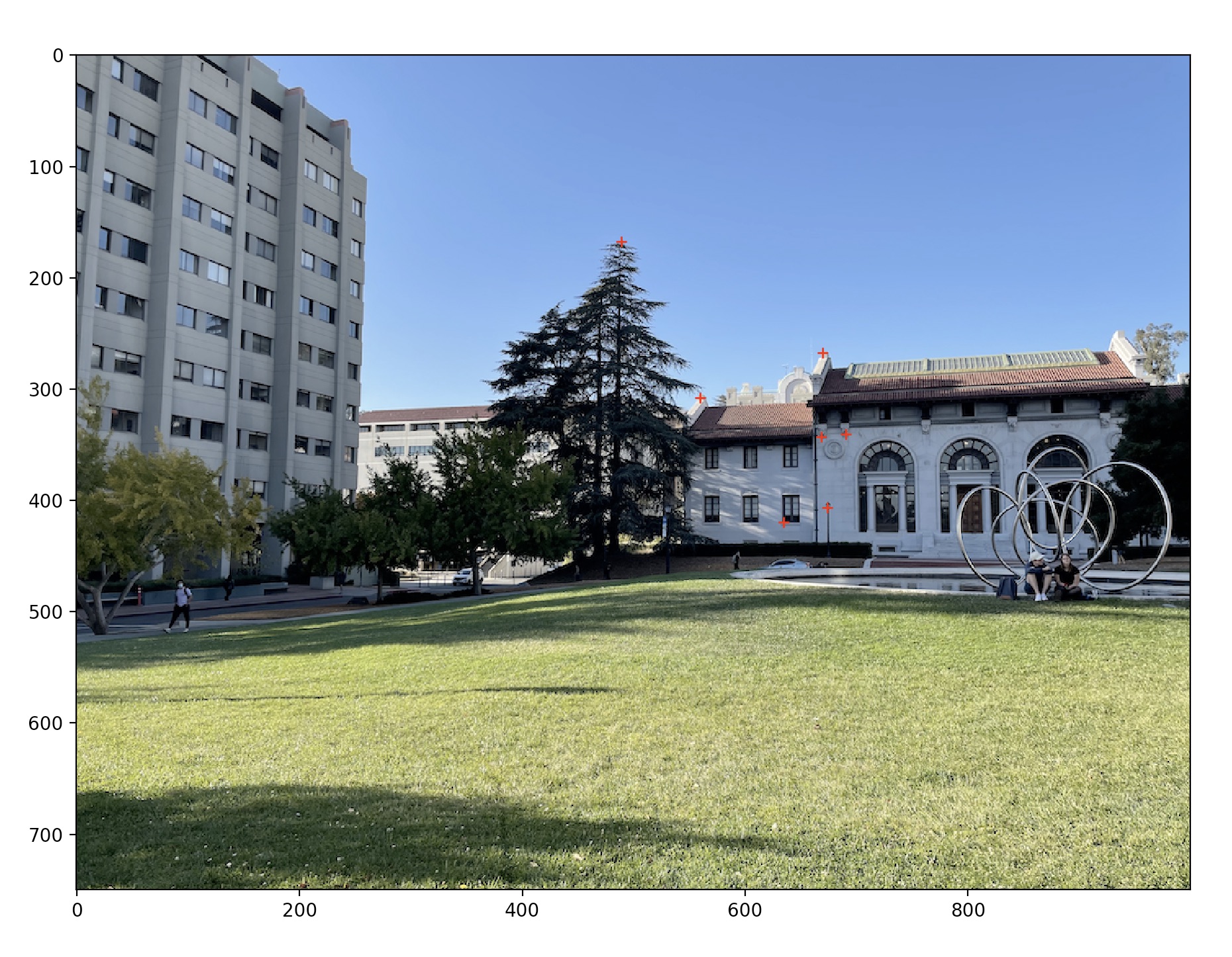
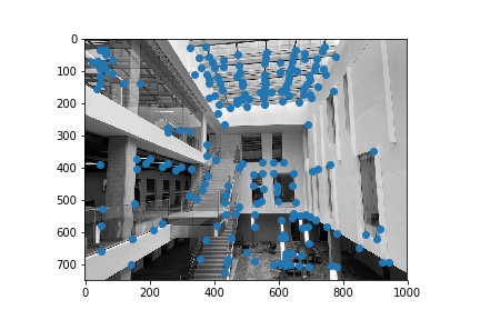
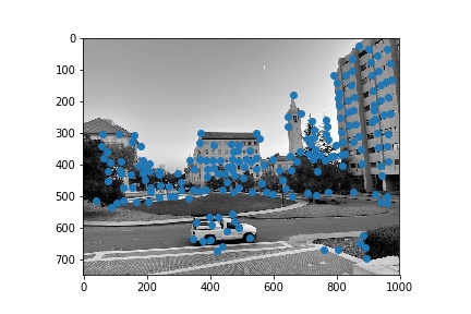
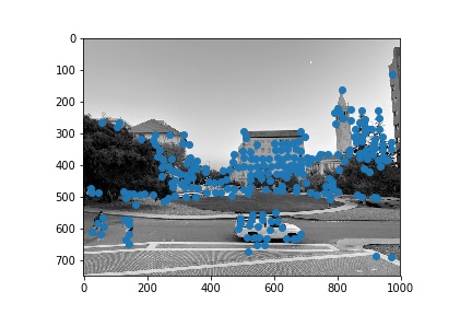
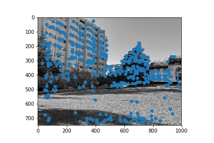
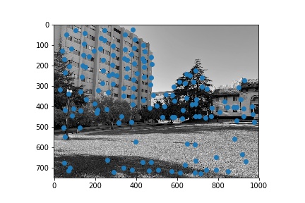
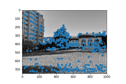
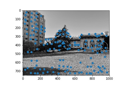
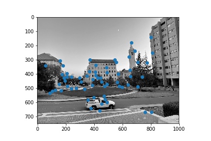
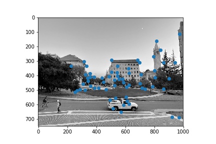
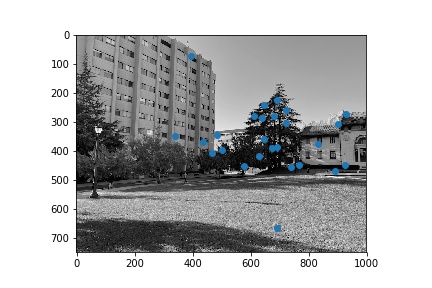
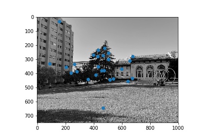
Using the algorithm for Harris corners, I generated several corner points on the image and then restricted it to the corners with the top n supression radii, where n was a variable threshold that varied for each image. Here are some examples of Harris corners generated, followed by the AMNS points.

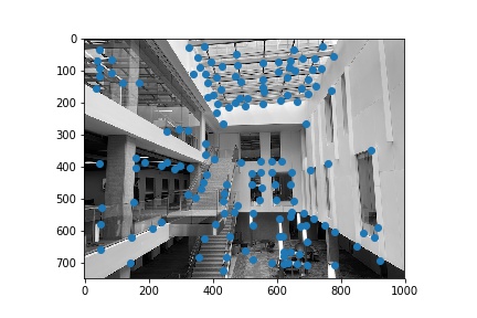


Here's the 40x40 sample (this point is the roof of one of the buildings in the Hearst Mining Building Steps photo, and then Gaussian blurred)

Here's the 8x8 downsample.

Then, I generated a feature descriptor for each feature point. I did this by looking at the 40px by 40px window around each feature point, and downsampling to get an 8x8 square instead. I then normalized it to account for changes in brightness and intensity. Here is an example below.
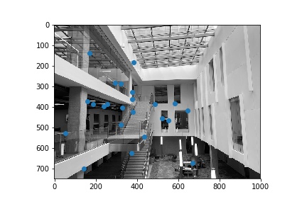
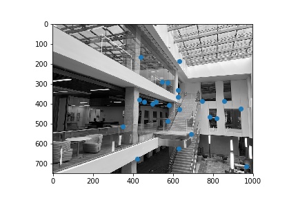
Then, match points by comparing their respective feature descriptors using the SSD.
A correspondence is defined between two points if the ratio of the SSD error for the two descriptors and the SSD between the descriptor for the second-best match is less than a user defined threshold; this varied per image but usually was between 0.1 and 0.3. The use of the ratio rather than the single smallest SSD ensures that the feature selected as a match was a significantly better match than any other possible point. Any point without such a match was discarded.
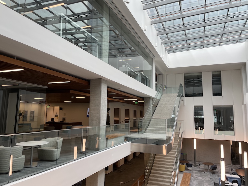
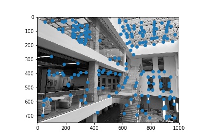
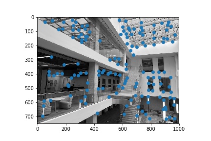
Below are the orignal points considered on each pair of images, followed by the points on the same images that were deemed to have a match in the other image.
After retrieving a set of at least four matches, we can compute a homography matrix. We use the RANSAC algorithm to eliminate the effect of any outlier pairs (pairs of points that were matched but do not actually map to each other in reality). For each iterations, 4 random points are sampled as input to calculate a homography. Using that homography, we calculate the correspondences for one image and we count the number of matched features that have a distance between the calculated correspndence and the matched feature that is under a certain threshold. This threshold was user defined, but usually fell between 5-20 pixels for each image. After recomputing a final homography matrix between all of the matched features, the images are stitched together.
After calculating the best-fit H, we use that to merge our images, using the same algorithm as Part A. Here are some of my results!
Here is the manually stitched panorama using the same images for comparison:
Here is the manually stitched panorama using the same images for comparison:
This part of the project was also super cool! I was actually kind of surprised my code ran as fast as it did, considering how many RANSAC iterations I had to do for each image. Overall, I think the photos came out looking great, and with much less work on my part for point selection :)