Recovering Homographies
In order to transform points between any of the images, we need to compute a homography matrix.
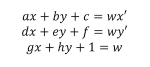
The homography matrix is defined as the matrix H that allows us to relate a set of corresponding points in the images.
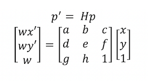
In the equation above, p represents a point in your first image and p' represents a point in the second image scaled by a factor of w.
The bottom right value in the matrix of H is set to 1 as it determines the scaling factor.
To find the homography matrix, we need to solve for all the remaining values in the H matrix. To do so, given we have points from the first image (x, y) and points from the second
image (x', y'), we can solve for these unknowns by creating a linear system of equations.
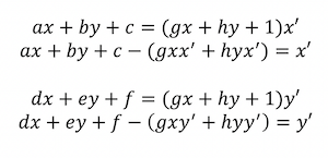
From the above equations, you get the below equations.
Rewriting the equations to isolate x' and y' on the righthand side, you get the below.
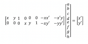
Given these, you can represent the H matrix unknowns as a vector and get the below.
Expanding this for n points instead of just one set of corresponding points, you get the below.
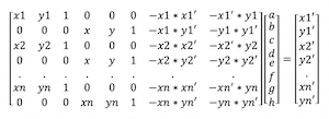
This gives a total of 2 * n equations that can be solved to determine the 8 unknowns in the H matrix. Given there are 8 unknowns, the number of correspondence points
you choose must be greater than or equal to 4.
It is best to have more than 4 points for the best results. I used around 10-15 for my images. Given more than 4 points, the linear system of equations is overconstrained and can be
solved using least-squares.
Once the unknowns are solved, you can reformat the unknowns vector into a 3x3 matrix with 1 in the bottom righthand corner and that is your homography matrix.
Image Warping
After computing the homography matrix, it can be used to warp images to another image's coordinate system. I used inverse warping to be able to determine the colors of the warped image from the original input images.
Given an image to be warped and a homography matrix H, I followed the below steps to create the warped image.
Computation Steps
1) Use the homography matrix H to find the warped coorindates of the image
2) Use cv2.remap() to map the colors of these warped coordinates to the original coordinates of this image in order to colorize the image.
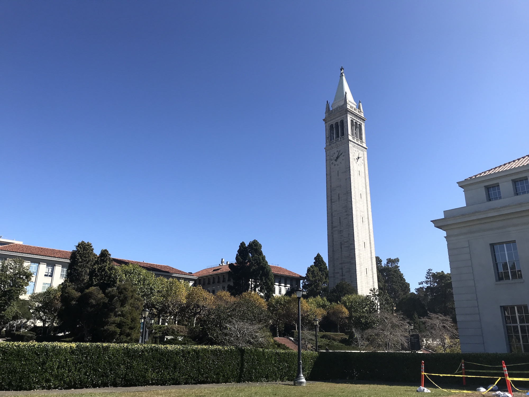
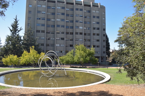
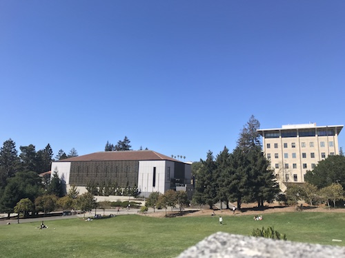
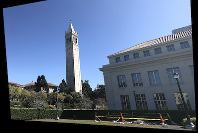
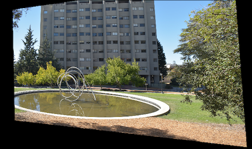
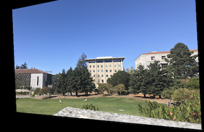
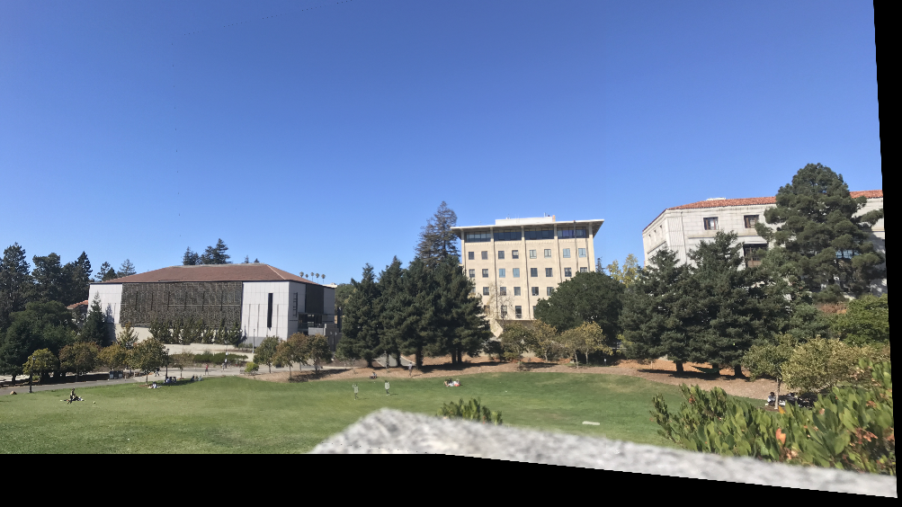
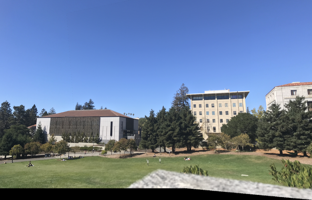
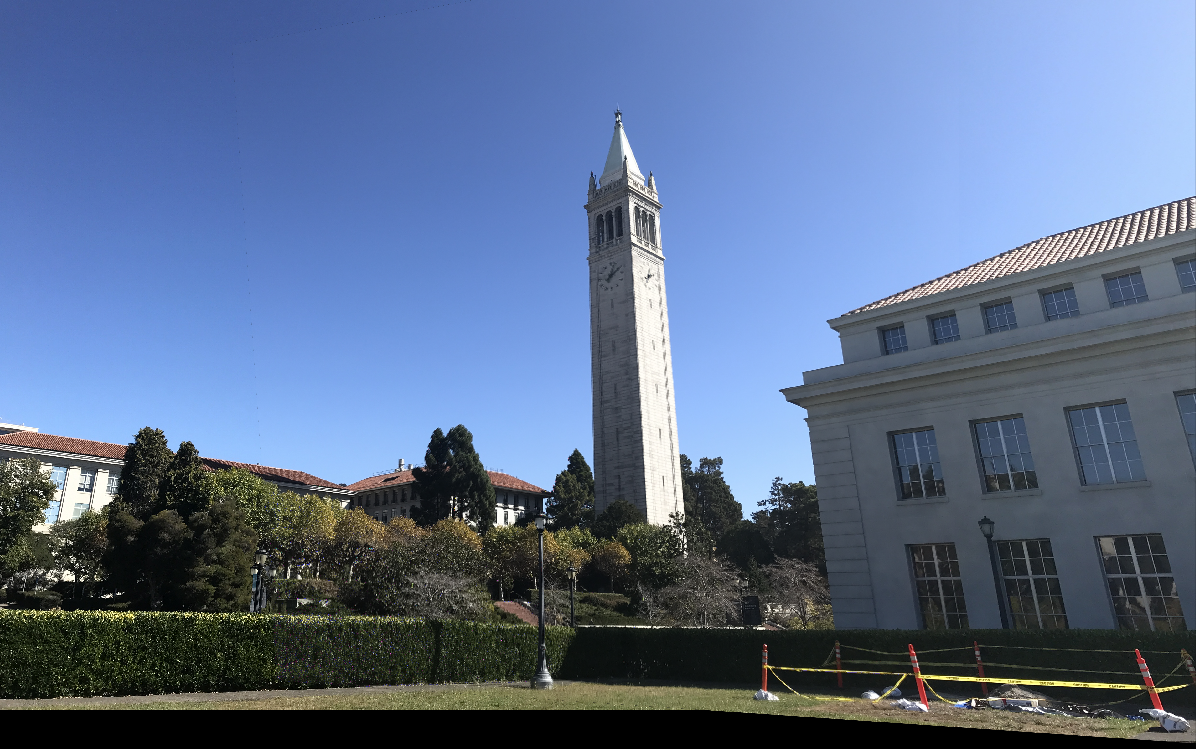
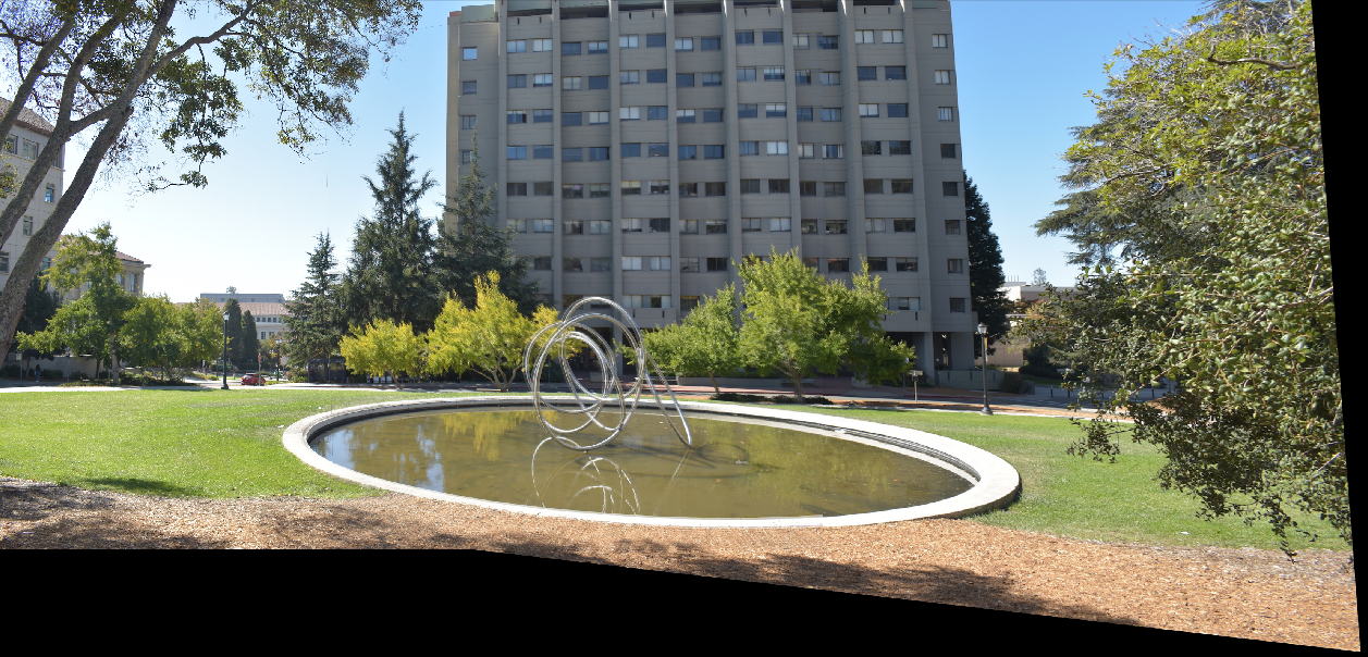
Below are some examples of warped images.
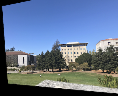
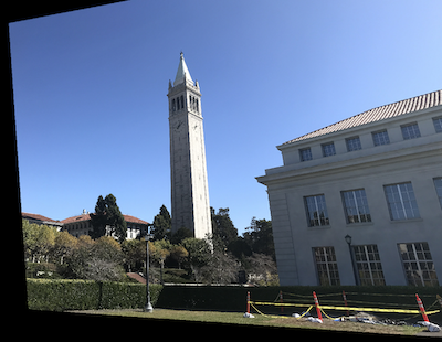
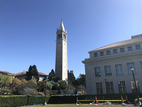
| Campanile (right) warped |
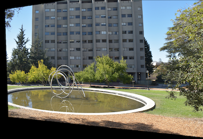
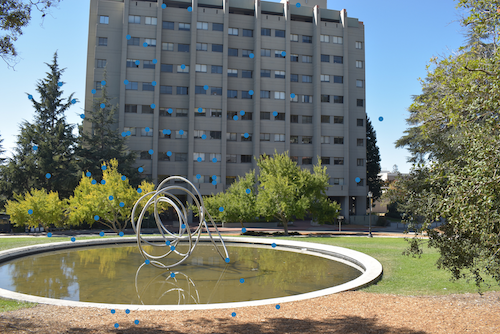
Hearst Mining Circle (right) warped |
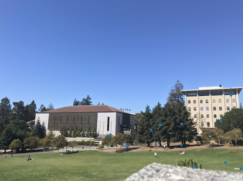
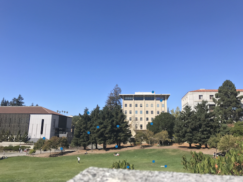
Memorial Glade (right) warped |
|
|
|
Image Rectification
With this image warping implementation, you can rectify images. Given an image with some planar surfaces, you can select feature points for this planar surface and warp
the image so that the selected plane is frontal-parallel.
I chose squares for my warps, so this meant that the "image 2" in the warp was just the coordinates of a square.
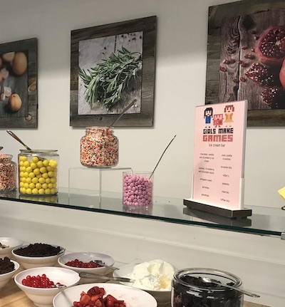
Below are some of the results of rectifying images.
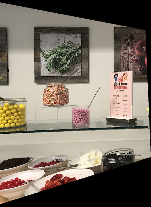
| Original Image |
Rectified using the square herb framed picture |
|
|
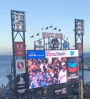
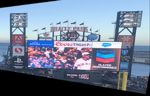
| Original Image |
Rectified using the Adobe sign |
|
|
Reflection (Part A)
The coolest thing I learned from this project was how simply warping an image can allow you to see an image from a different perspective as seen in the examples of image rectification.
Project 4 Part B
Feature matching for Autostitching
For part b of this project, I will be automatically stitching together images by implementing automatic feature matching.
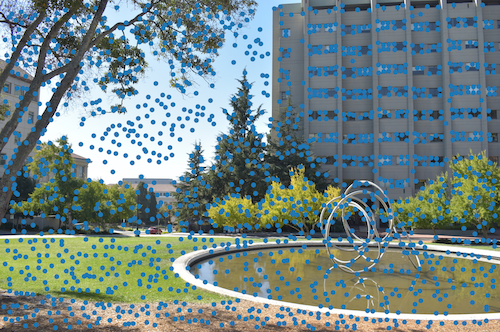
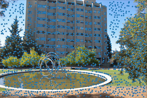
Feature matching
Now that we have our feature descriptors, we can match them. To match features, we want to take each of the feature descriptors
that we have from the first image and find the feature descriptor in the second image that most closely matches
this feature descriptor. We measure the similarility by calculating the 1-NN and 2-NN match in the second image for every feature in one image using
a sum of squared differences funciton. Once we get the SSD value between two feature descriptors, we check that this SSD(patch 1, patch2) < threshold.
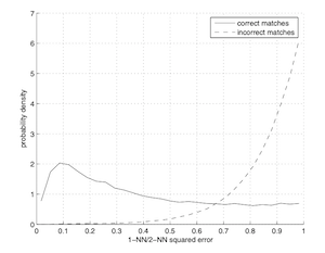
The idea is that the 1-NN, which is the SSD of the closest match (nearest neighbor), should be much better than 2-NN, which is the SSD of the second best match.
If the 1-NN is not a much closer match, it's likely that it is not a great match and we don't use it. This threshold concept is
based off Lowe's trick. The threshold can be determined by trial and error depending on how many incorrect matches
are acceptable in your situation. For me, I used a threshold of 0.2 since these mosaics can be very sensitive to incorrect matches and we don't need an extremely
large number of correct matches to create a good mosaic. As seen from the graph below, this avoids picking up a lot of incorrect matches.
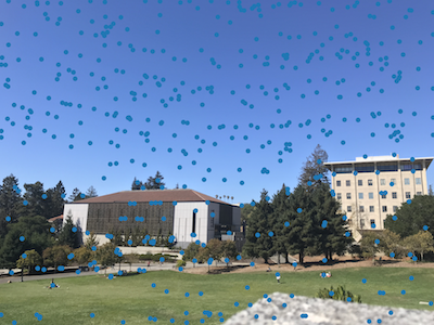
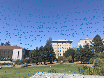
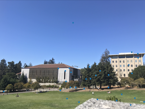
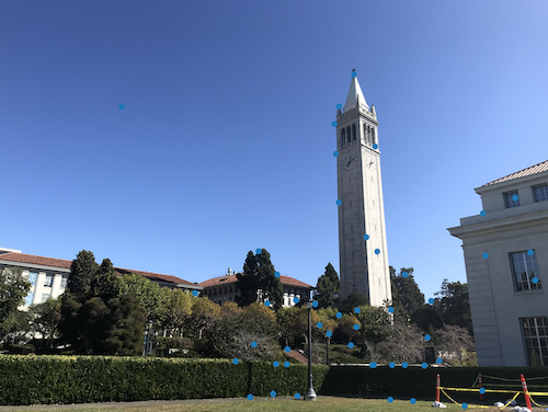
Below are the results after feature matching.
| Feature matches left |
Feature matches right |
|

|
|
|
|
|
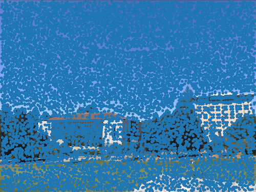
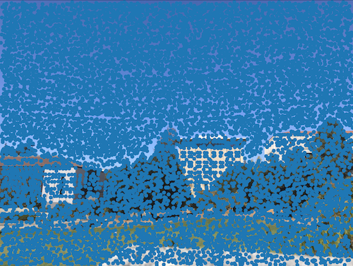
RANSAC
While feature matching does a pretty good job of identifying matching points, there's still some outliers in the images.
In the above images, you can still see some points in one image that either do not match to points in the second image because the
part of the image does not exist in the other image or are identifying features that are similar in appearance (eg. blue sky) but not in the same location.
To remove these outliers, we apply RANSAC. The steps followed are below.
Computation Steps, repeated N number of times:
1) Pick 4 random pairs of feature matches
2) Find the homography matrix for these 4 random pairs
3) Use this homography matrix and apply it to the 4 points from one image to transform them into the coordinate plane of the other image. Normalize these points.
4) Find the number of inlier points that have SSD(homography * point, corresponding point in other image) < error epsilon.
5) If this number of inlier points is greater than the current maximum number of inlier points, set these points as the maximum set of inlier points.
After N iterations, take the maximum set of inliers and use these to calculate the homography matrix. I chose an N of 4000.
Now, we can use this homography to do the same warping and blending steps we did in part A of the project.
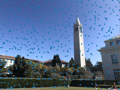
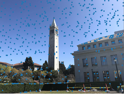
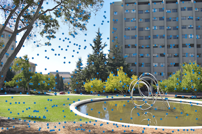
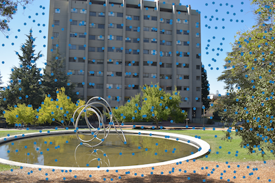
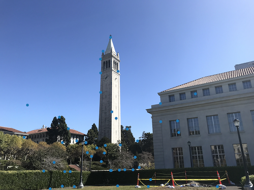
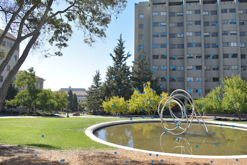
RANSAC points
| RANSAC matches left |
RANSAC matches right |
|
|

|
|

|

|
As you can see, the outliers in the sky/other weird places have been filtered out by RANSAC.
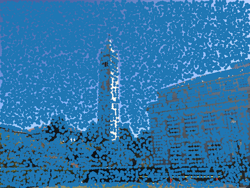
Warping these RANSAC images
Comparing auto and manual point selection results
| Manually selecting points result |
Auto selecting points result |
|
|
|

|
|
|
Evidently, the automatic image matching does a better job (there is less blur in most images).
Reflection (Part B)
My favorite thing I learned from this project is how we can remove outliers and drastically improve the results with Lowes trick/RANSAC. They might seem like non-crucial parts of the project but both
made a huge difference in my results.