CS 194 Project 4: Image Warping and Mosaics
Zachary Wu
PART A
Shooting the Pictures
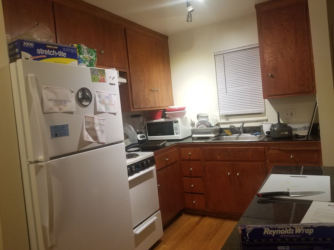
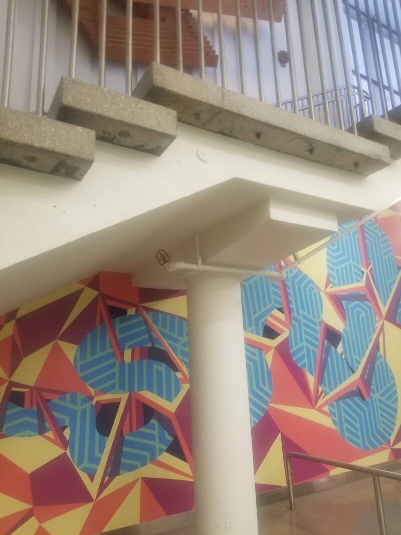
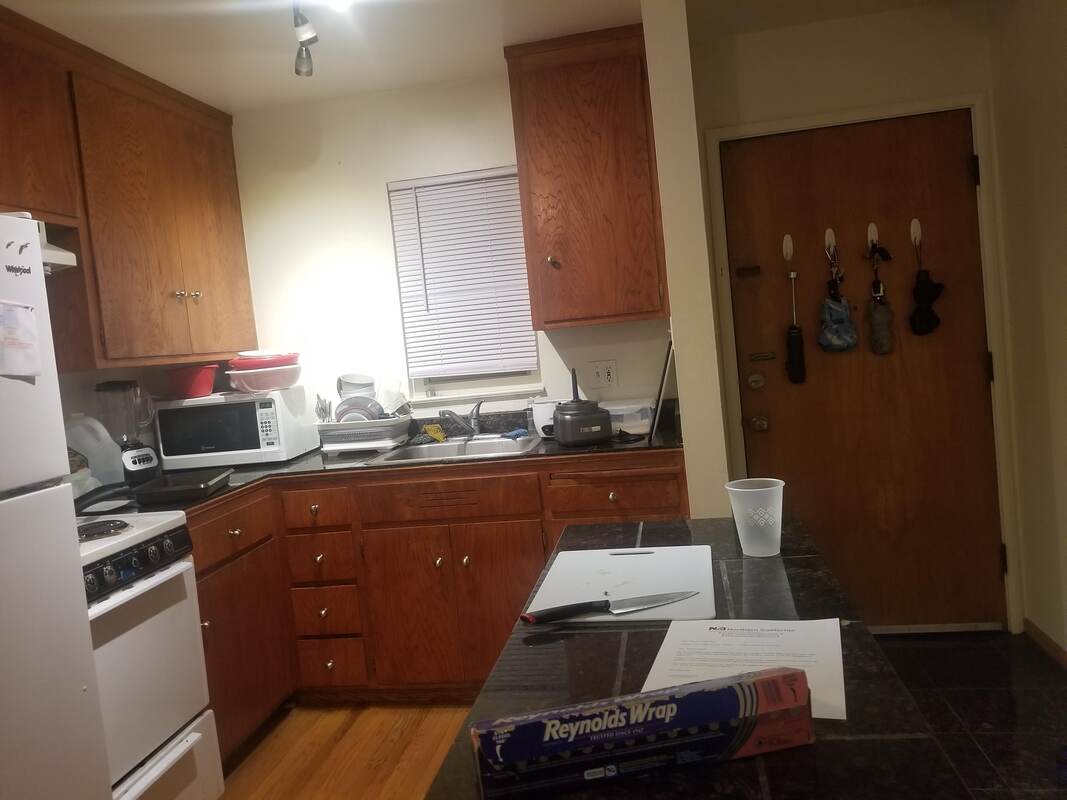
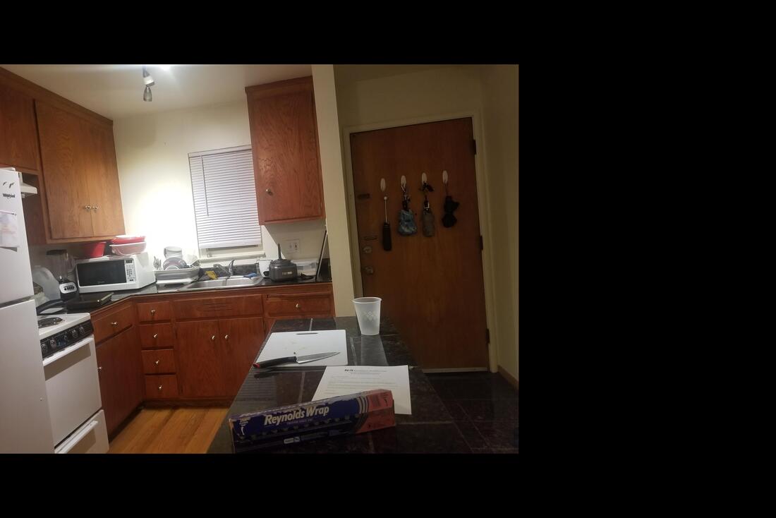
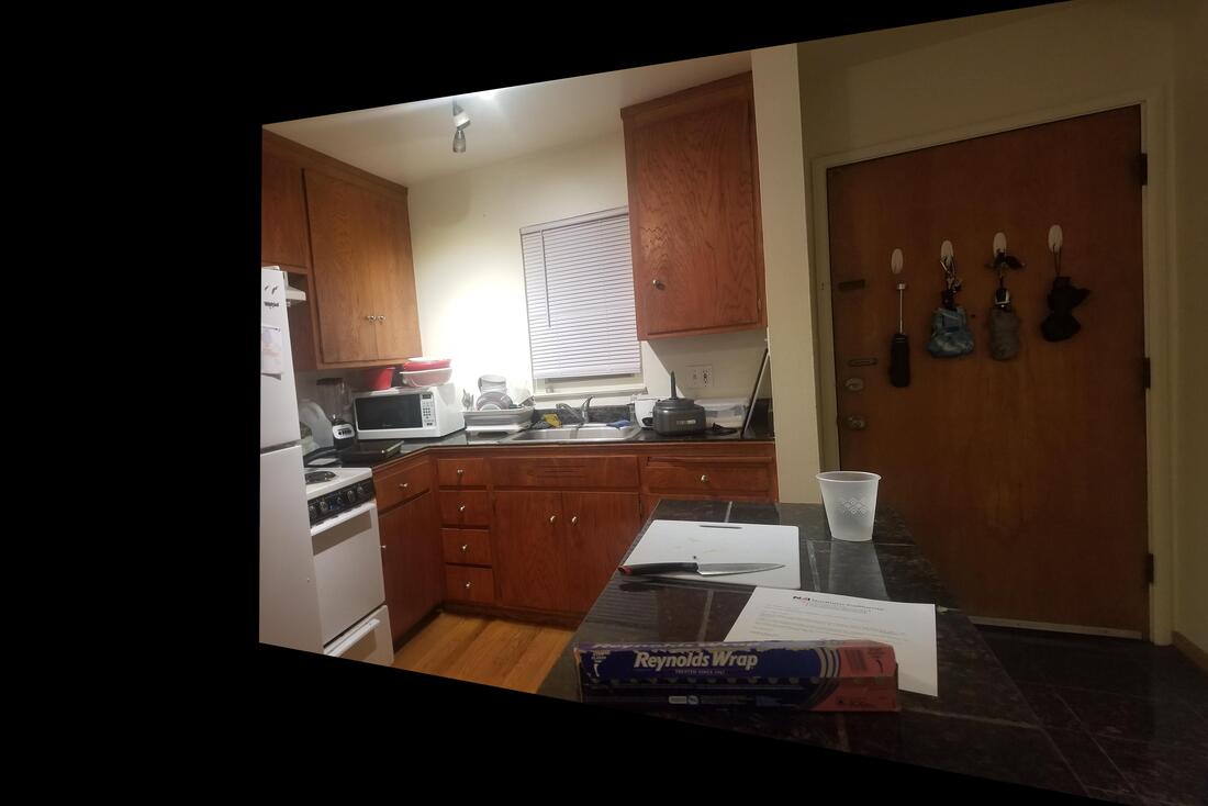
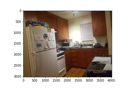
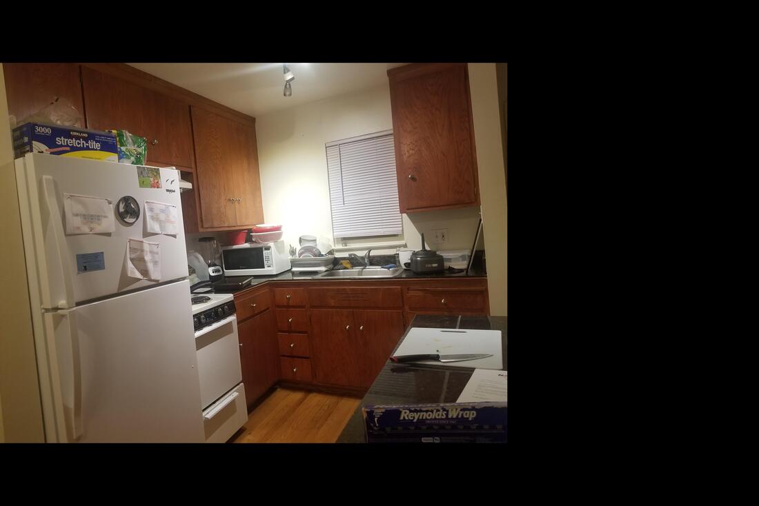
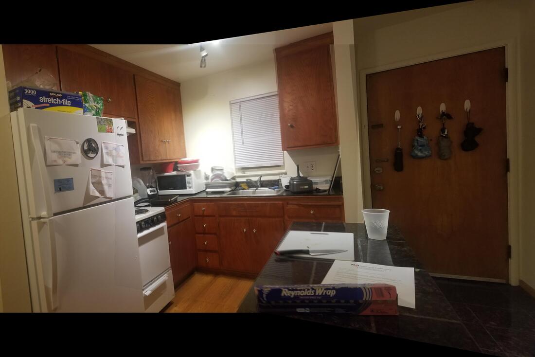
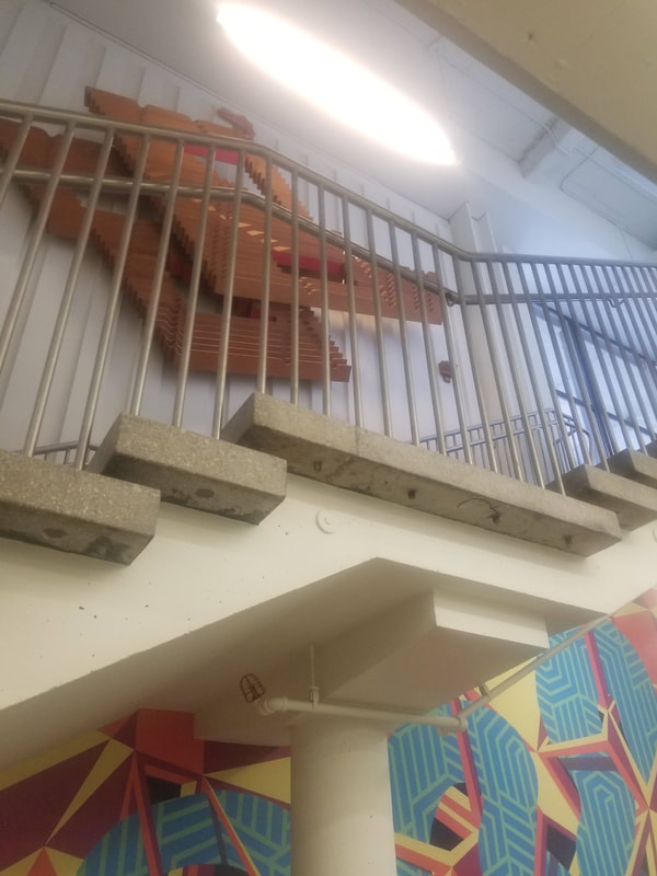
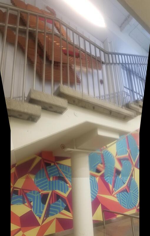
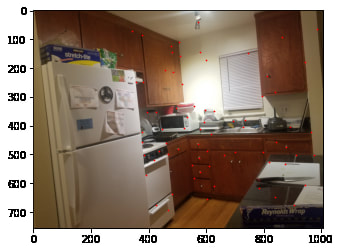
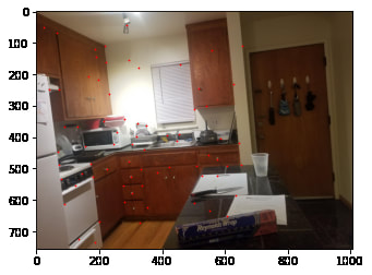
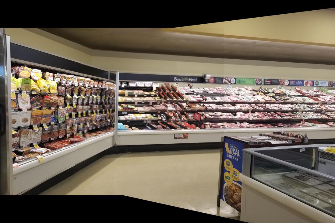
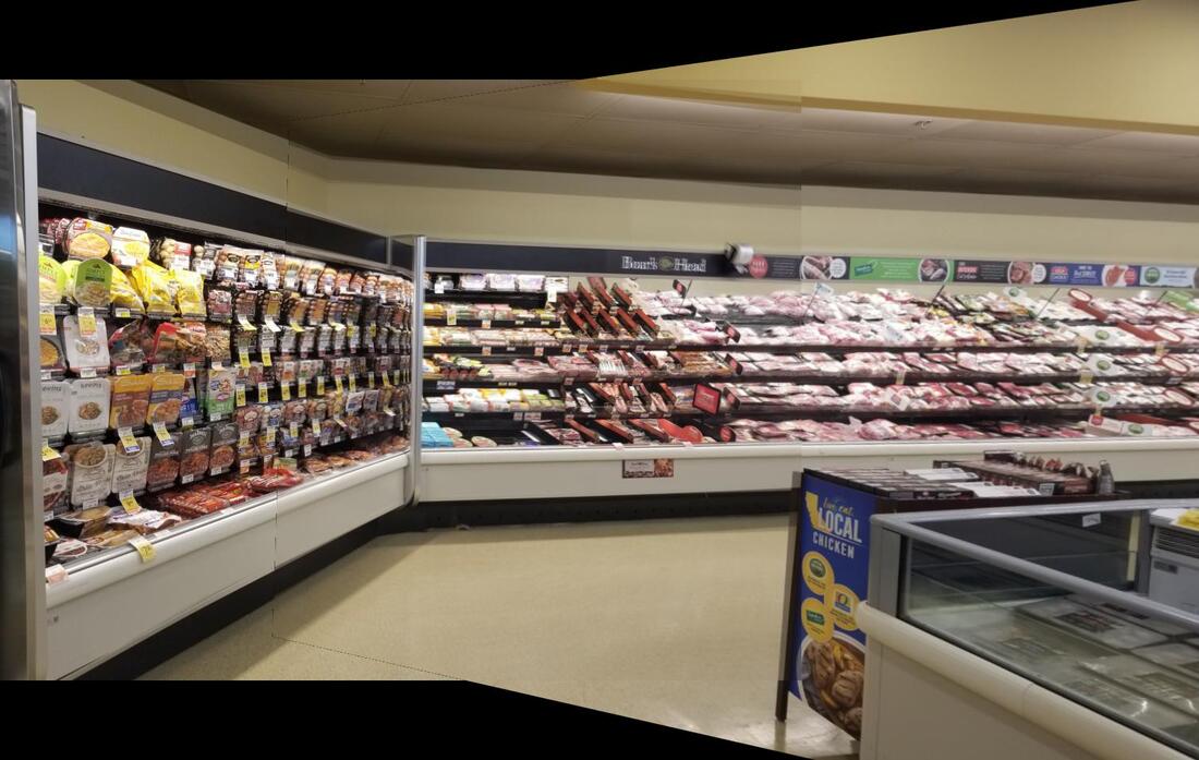
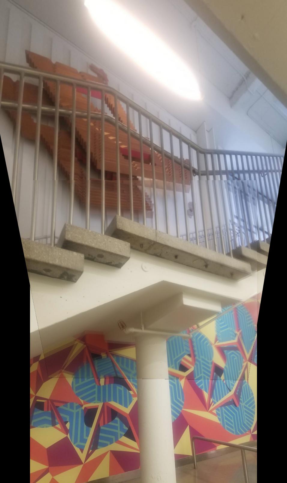
Using modern technology, shooting images is incredibly easy. Using my phones built-in camera, and a tripod, I captured multiple pairs of images of my kitchen, Safeway, and stairs within MLK. The goal is for each of these images to have perspective transformations between them. In this case, this is achieved with a tripod to maintain the same point of view, but different view directions.
|

|
Recover Homographies
Going forward, I will use the image of my kitchen to showcase how the process works.
We will now try to compute the homography between the images. This tells us the perspective transformation that takes place the two images. We will compute a 3x3 matrix H, that when multiplied with one of the images, will align it with the other one.
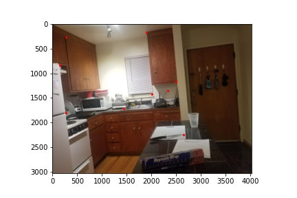
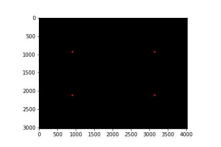
In order to solve for the homographies, we first have to manually identify at least 4 points of correspondence. Below, I have manually selected some correspondences between the two images on sharp corners that both images share.
We will now try to compute the homography between the images. This tells us the perspective transformation that takes place the two images. We will compute a 3x3 matrix H, that when multiplied with one of the images, will align it with the other one.
In order to solve for the homographies, we first have to manually identify at least 4 points of correspondence. Below, I have manually selected some correspondences between the two images on sharp corners that both images share.

|
|
Using these points, we can set up a system of linear equations and do least squares to get the best H matrix that will result in a clean transformation that aligns the matching points. I used this math stack exchange answer, and this towards data science article to help learn about this process, and will summarize them below. Equations are from the article.

First, we start with a set of at least 4 pairs of points that correspond to before and after the transformation.

Our homography matrix H, multiplied by the original points will get us the final desired points. In order to solve for H, we have 8 unknowns (with h_33 being 1). Using 4 pairs of points allows us to get 8 equations. In this case though, we will use more points, and use least squares to have a better holography, as manual selection of points can be quite hit or miss.
Shreyans Sethi explained how to derive the equations on piazza, which I will quote here.
"""
Expand the original equation, we will have
ax + by + c = wx'
dx + ey + f = wy'
gx + hy + i = w
Now, because all the RHS's of the above equations share a w, you can sub in the value of w to get
ax + by + c = (gx + hy + i)x'
dx + ey + f = (gx + hy + i)y'
Expanding this out will get you:
ax + by + c = gxx' + hyx' + ix'
dx + ey + f = gxy' + hyy' + iy'
"""
This ultimately gives us a least squares problem that looks we can solve for the 8 unknowns for.

In the case of my kitchen picture, I receive the following resulting H matrix
[[ 6.31290874e-01, 6.41588866e-03, 1.30776077e+03],
[-1.26032049e-01, 8.83592102e-01, 1.27723401e+02],
[-9.77570199e-05, 9.27963080e-06, 1.00000000e+00]]
[[ 6.31290874e-01, 6.41588866e-03, 1.30776077e+03],
[-1.26032049e-01, 8.83592102e-01, 1.27723401e+02],
[-9.77570199e-05, 9.27963080e-06, 1.00000000e+00]]
Warp the images
We can now use our calculated homography matrix to warp our second kitchen image to match up the correspondance points with the first matrix.
To do this, we take each possible index and multiply it by the Homography matrix (or inverse depending on which image we are changing. Then we use cv2 remap to interpolate the colors from the image into it's new positions, and this gets us the warped image.
We also begin with some padding such that after the perspective transformation, we still have all the pixels and the images are not cropped.
|
|
Image Rectification
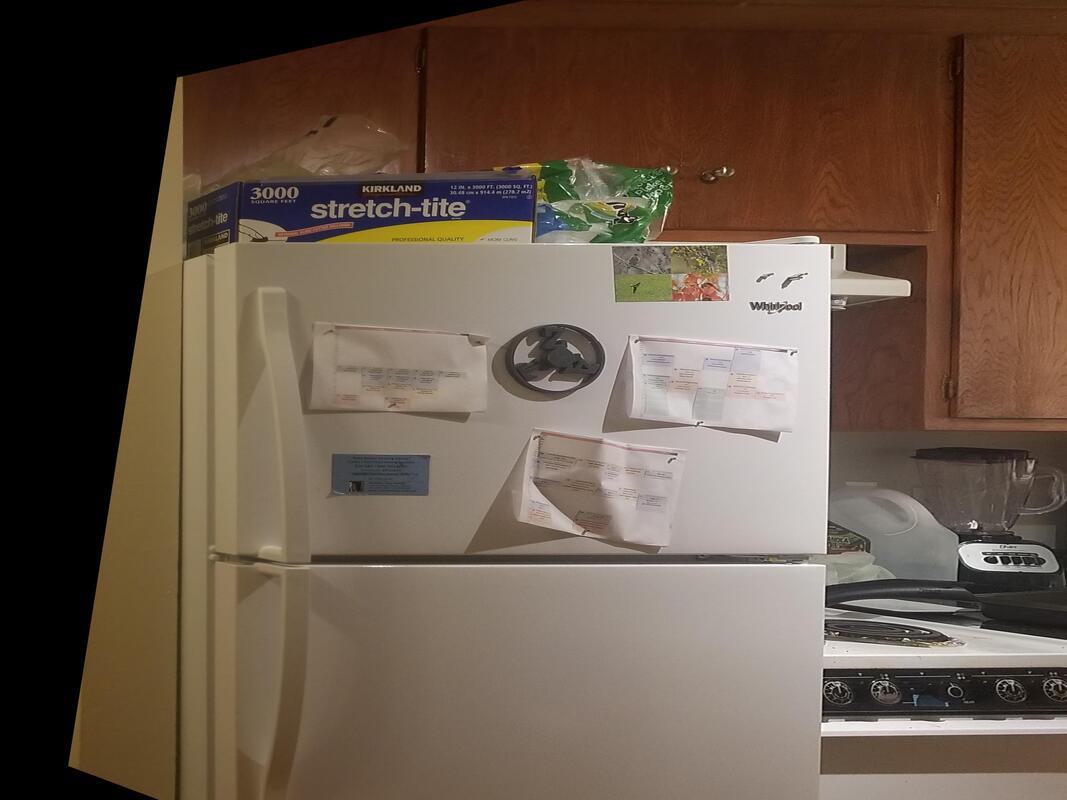
One great thing about being able to warp images is we can rectify images to be as if we are viewing them from a different point of view. For example, consider the our kitchen image. What if we wanted to be able to read the things posted on the fridge head on?
We can simply use correspondences to transform it to be head on. First I define correspondences for the area of interest, and set it to become square in the perspective that we want.
We can simply use correspondences to transform it to be head on. First I define correspondences for the area of interest, and set it to become square in the perspective that we want.
The 4 corners of the fridge
|
A square head on perspective of viewing the fridge
|
Now using the same steps of computing homographies and warping the image, we get the following result.
|
|
|
Now we can read what is on the fridge head on! However, do note that the picture is a bit blurry, as rectifying the image does not allow for sharp images, as previous pixels need to be stretched, making certain parts appear blurry. You can't create pixels that aren't already captured in the original image.
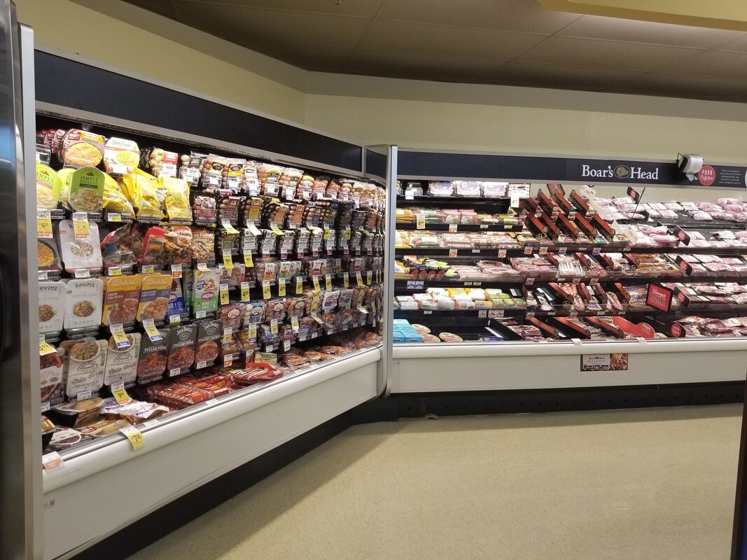
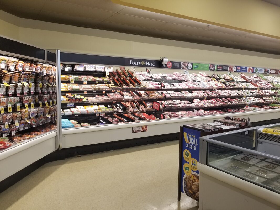
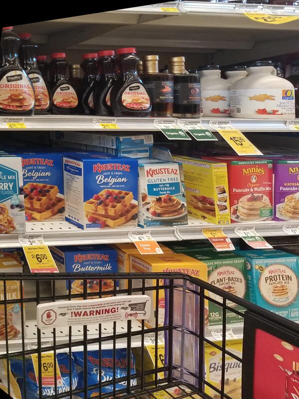
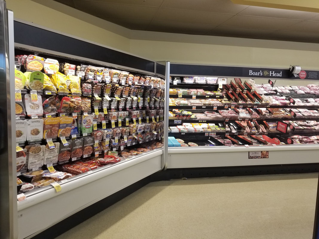
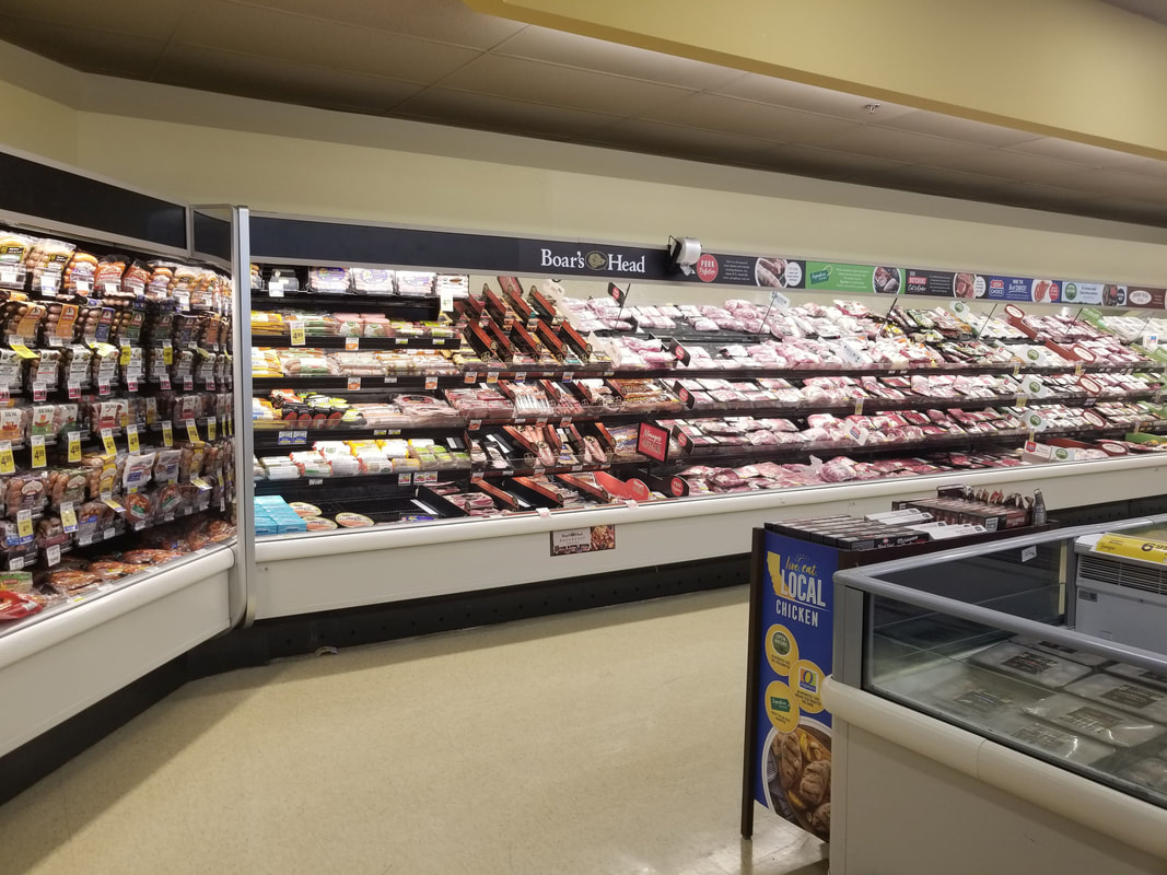
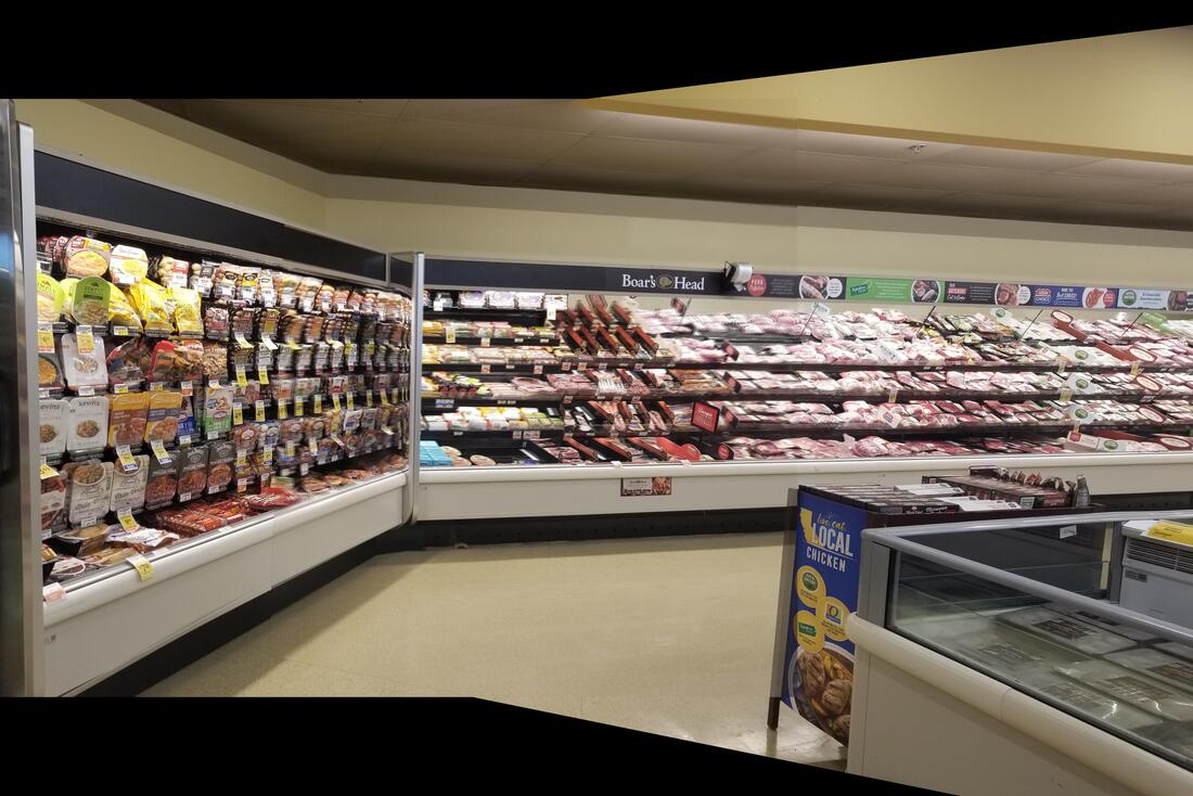
Here's another example of rectifying an image in order to browse the breakfast isle at Safeway.
Here's another example of rectifying an image in order to browse the breakfast isle at Safeway.

|
|
While image rectification is great for changing our perspective, it is not magic, and we cannot change our viewpoint to one in which we see things that the original picture does not capture.
Blending Image Mosaics
We now have two images of our kitchen, that are lined up, and we need to blend the two of them together.
|
|
The first blending method I will do is to to simply add the two images together. This will cause the overlapping portions to be incorrect. To correct this, we will create a mask for the overlap region, and in that area have .5 of each image.

The result is quite good! although there are some slight artifacts in the overlap region where we see some mismatch and a some subtle lines from the blending. The edges not matching up perfectly is most likely a result of the lens distortion on my camera making the image plane not perfectly flat.
Now, we will show 2 more examples of creating a mosaic.
Now, we will show 2 more examples of creating a mosaic.
|
|

|
|
What I Learned
For this part, the coolest thing I learned is being able to rectify images and create get an image from a new perspective. It allows an image to be created that was never taken, but you can still see if from a differnet perspective.
PART B
We have now covered the process for creating panorama pictures and other mosaics. However, the process is quite inefficient. It requires a human (me) to manually select and match points, which is infeasible when we have many pictures that we want to stick together. To fully make this whole process more automatic, we will attempt to implement automatic feature matching to find correspondences from the pictures themselves. no input from me required.
Many of the ideas for the part of the project come from this paper by Brown et Al.
Many of the ideas for the part of the project come from this paper by Brown et Al.
Harris Corners
When matching between two images, corners are often very good to select. Corners serve as sharp distinct features that vary in all directions. On the most basic levels, Harris corner goes through the image and windows of pixels that change greatly in both the x,y directions. This is a property that only corners will hold, and one that edges or a neutral background will not.
For the specifics, please refer to these slides from class, starting on slide 19.
For our project, we were thankfully given code that finds Harris corners in an image, and the corresponding h values of each point that corresponds to how strong of a corner that point is. Using this function, and removing all of the points with a small h value (not strong corners), a large number of potential points of interest for our image.
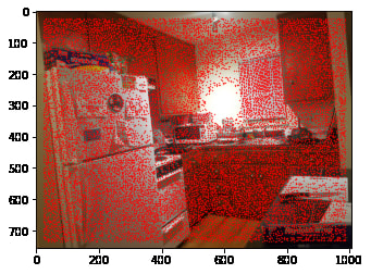
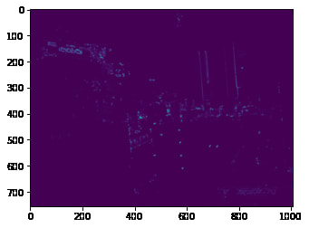
We can also display the h values across the image, which identifies areas with sharp corners. We see that the knobs on the cabinets do very well to serve as potential features to be matched on.
ANMS
Unfortunately, we can't just use every single Harris point that we found. There are way to many of them (~39k) which will make matching difficult. Additionally, not all of them are great corners.
To filter them down, we can do something as simple as taking the n points with the strongest h values. However, this tends to cluster points in certain regions, which may miss parts of the image, messing up our homography if there are no good overlap points.
In order to address this, we use ANMS (Adaptive Non-Maximal Suppression) details of this are outlined in the paper by Brown et al. The algorithm works by calculating for each point a radius, in which that point is the maximum compared to those around it. It then takes the n points with the largest radius. The idea is that we will both pick very strong points, because it will have a high h value, and thus be the largest point in a large radius. This algorithm will also points in areas without many corners since the strongest point there will have a large radius. By doing so, we are able to get an very even distribution of points across the image, with each point being and approximate local maximum to avoid too much information in any particular area.
After doing this and picking the 250 strongest points, we are left with the following points.

Extracting Feature Patches
Now we extract features from the selected points. These features will be 8x8 patches around each point selected above. For this project, we will not worry about rotational invariance, since the images were taken on a tripod.
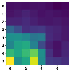
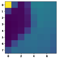
For each point, we begin with a 40x40 patch of pixels. We downscale this to 8x8 though, essentially applying a blur and removing some high frequencies. We do this to "give the features some robustness to interest point location error". Each patch is also normalized to mean 0, std 1 so that they are not dependent on luminance or other differences between the two iamges.
2 examples of patches we take from the image, and the corresponding downsampled feature patch are given below.
|
40x40 windows around 2 different harris points


|
8x8 downsampling of the feature window, normalized
|
Feature Matching
Now that we have 250 features for each of the images, we need to match up the features together. To measure similarity from two features, we will use the Sum of (SSD) sum of squared differences as a measure of error between the two.
The simplest algorithm is to pick the nearest neighbor for each feature in image 1, that is the corresponding feature with the lowest SSD. Then we can simply set a threshold and select matches that have low error between them.
A more robust way that is implemented in this project however is to calculate the ratio for the error between the 1-NN and the 2-NN. This way, we can pick not only two features with low SSD, but also ensure that they are matches in which there are no other potential good choices.
After doing this matching, we get 250 matching pairs with the following ratio distribution
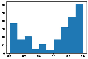
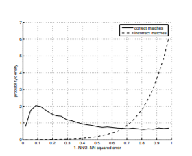
This looks very similar to the one presented in the brown et al. paper which is promising. While we can't distinguish correct and incorrect matches, we will assume that the underlying shape is correct, which allows us to set a cutoff at 0.3 that does a good job of keeping true matches, and eliminating false positives.
Looking at the matching points we keep below, it does appear at an initial passthrough that they are all indeed matching points for the most part! for every point in 1 image, we can easily identify a point in the other that is a pretty good match.
Looking at the matching points we keep below, it does appear at an initial passthrough that they are all indeed matching points for the most part! for every point in 1 image, we can easily identify a point in the other that is a pretty good match.
|
|
Computing Homography with RANSAC
Lastly we will compute our homography. But not so fast. While the previous steps are relatively robust, we may still have some matches that are incorrect.
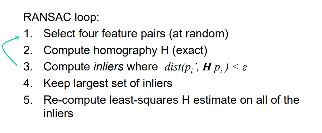
In order to deal with this, we use random sample consensus (RANSAC). The idea is we take a random set of 4 matches and assume they are correct. We then compute homographies, and check how many of the other matches are within a small error (set at root(2) to be within one pixel) compared to the homography applied to the original points. These points are called inliers, as they agree with the random sample we choose.
We loop through this multiple times, keeping track of inliers, and pick keep the matches for the set of largest inliers that all agree together. incorrect matches will thus be filtered out this way, as they will not agree with most of the other points.
Pseudo code for the algorithm is as follows
Then we simply compute a new homography using least squares on the largest set of inliers we have found.
Then we repeat what we did, and form some cool mosaics!
For the kitchen picture, my algorithm found a set of 49/72 points that all agreed on a homography. Using these matches, we calculate the following homography matrix.
[[6.10864694e-01, -4.35038345e-05, 3.28580724e+02],
[-1.33895981e-01, 8.74893103e-01, 3.40771286e+01],
[-4.11747103e-04, 2.66272898e-05, 1.00000000e+00]]
AutoImage Mosaics
Now with our homography matrix, we can repeat what we have earlier and create mosaics! Results below will compare the mosaics with manual selection to automatic feature selection.
Manual Points Selection
|
Auto points Selection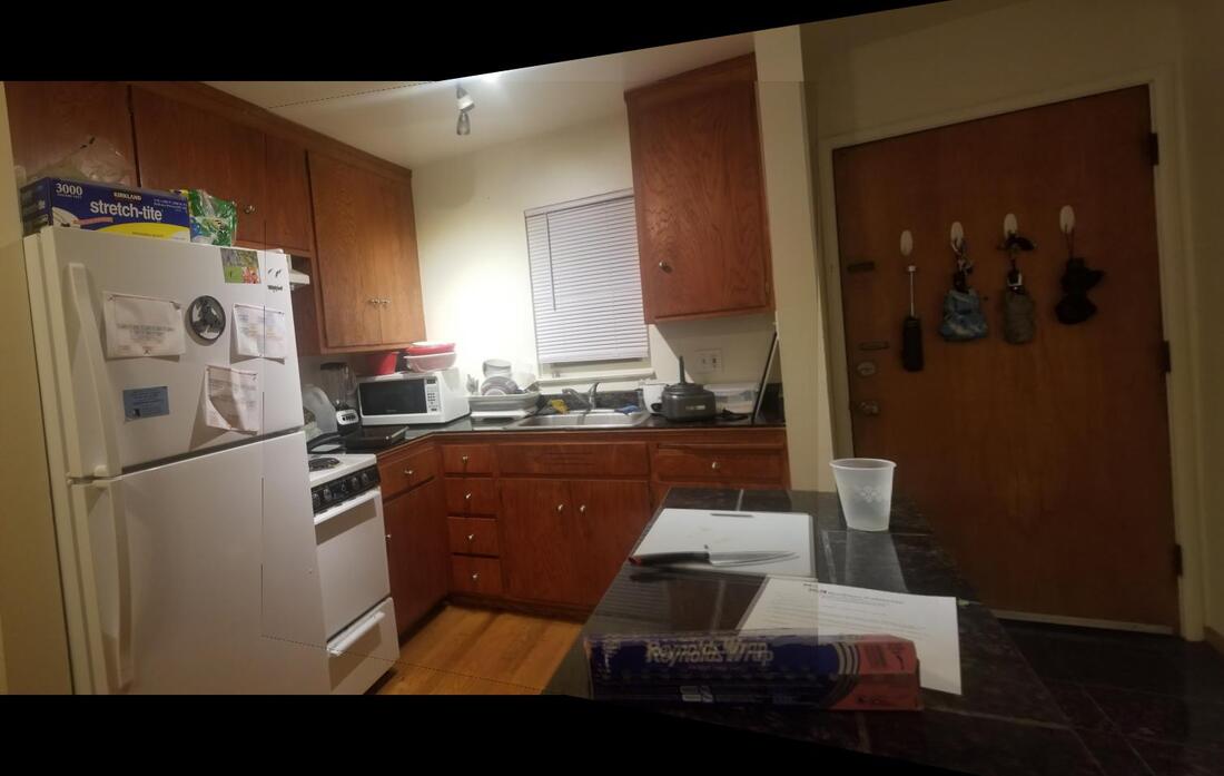
|
|
|
Looks pretty good! For the kitchen, it looks like it actually did a better job than me, as the artifacting near the edges (probably due to lens distortion) appears to be better. The grocery picture is about the same. However, the stairs picture is a vast improvement! It looks like I selected a poor set of correspondances, and autoselection was able to select one that resulted in a much better overlap and cleaner blend than I did.
What Have I learned?
There were many cool things I learned in this project. These include:
- Finding Homographies between two images
- Transforming and blending images to form mosaics
- Using Harris Corners as a means of identifying features
- Adaptive Non Maximal Suppression instead of a naive algorithm to best select feature points
- Intelligently feature matching based on ratios between nearest neighbors
- RANSAC as a means to eliminate bad matches