Part a: Image stitching

Overview

The purpose of this project was to stitch together images taken from different angles to create one contiguous parnorama shot. I did so using the principle of homogenous matrices, image warping, and image combination / blending!

Shoot and digitize pictures

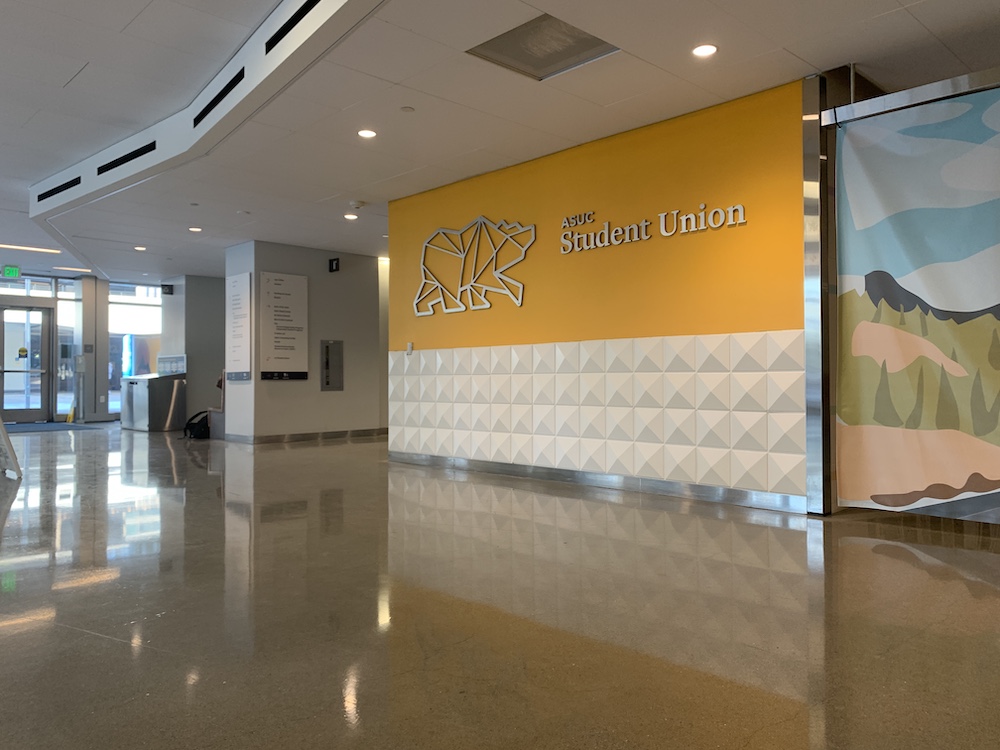
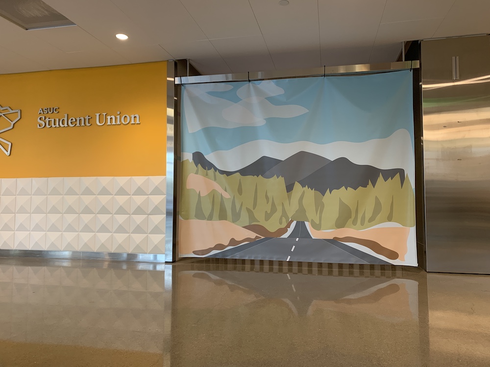
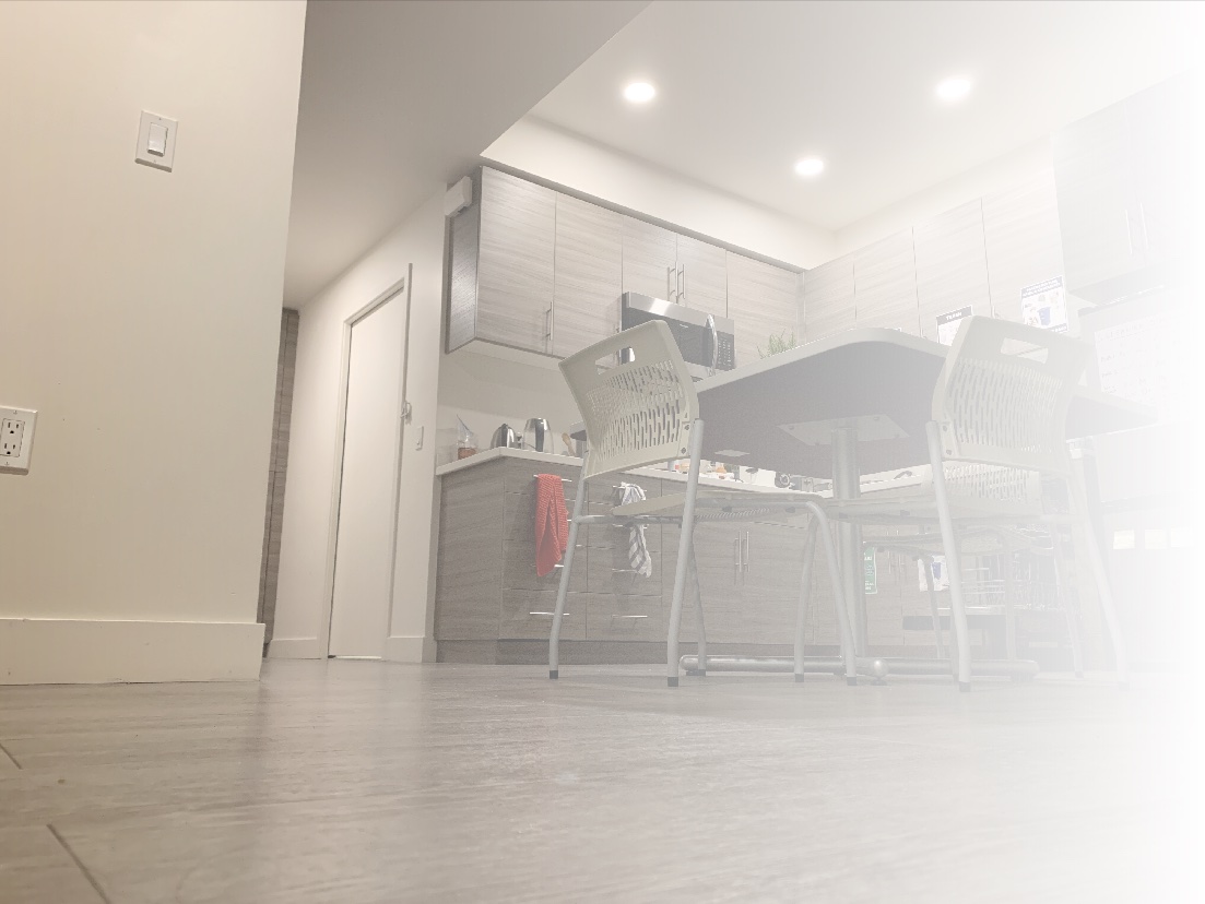
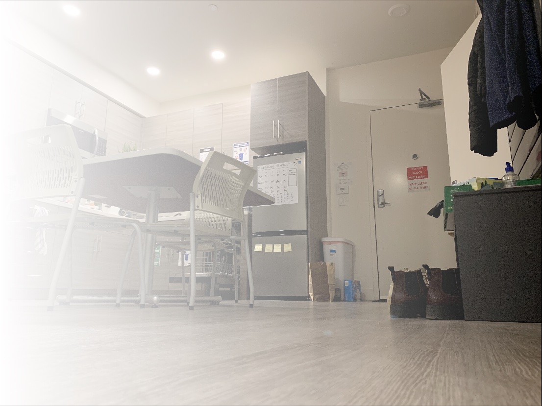
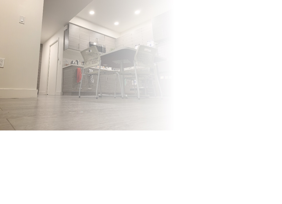
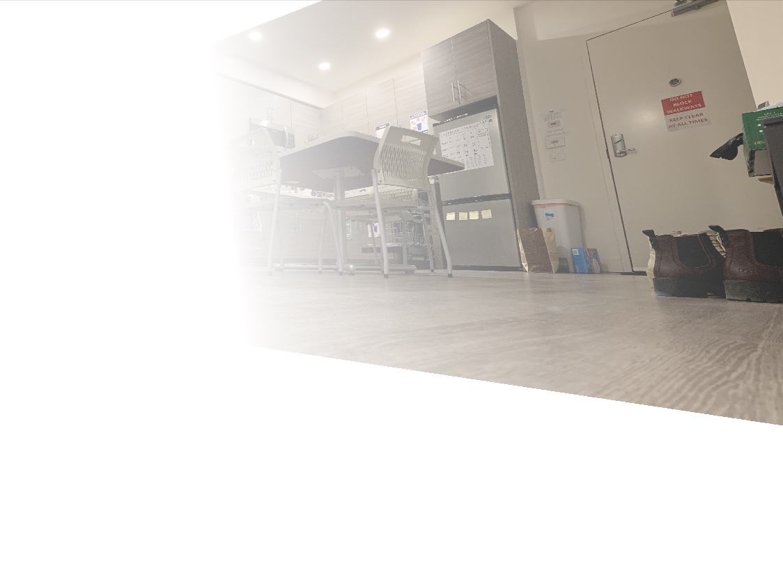
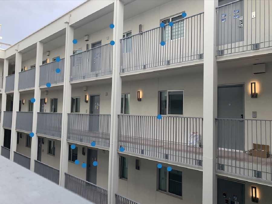
I first took some photos of my surroundings! These were taken with my camera staying still and with the iPhone exposure locking feature activated. As I did in the previous project, I stored my keypoints for each image as an array in text files, using the save_image_to_file function. To access these points, I used get_point_from_file -- this allowed me to only define and generate my points only once, which saved a lot of time when debugging an generating images! Here are the images I shot and used for this project:

Recover homographies

A homography is used to warp one set of keypoints to another. This useful to define a relationship between two images with given keypoints so we can warp images to align with one another. In order to compute the homography, I use the relationship that A*h = b, where A defines a a set of equations for each keypoint given, b is the transformed points, and h is a 1x8 vector corresponding to the flattened homography. Here is the math I used to solve for the system of equations to solve for A:

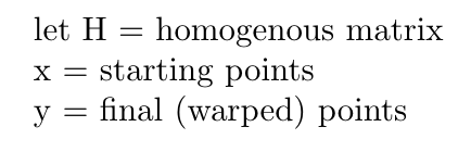
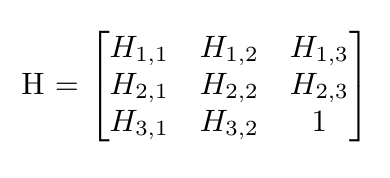
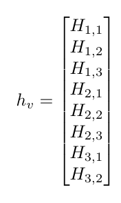
In this case, we let the homography matrix be defined as such (note that the bottom right corner is a scaling factor, established to be 1):

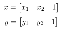
We want to use our H matrix to warp the points in x to points in y using the following vectors, given that H * x = y.

In order to solve for the values in the H matrix, we can use least squares! So, we can create a system of equations to solve for these values, and construct an A matrix and b vector to solve for them! In order to put H in the correct format, we must stack every element on top of each other as such:

After doing some equation manipulation, we result at equations of the form

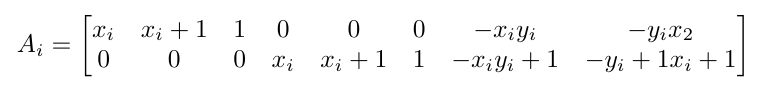
in the A matrix. For every i, these matrices of A would be stacked on top of each other! For every y value, you can also stack the b's into a vector of the y points as such:

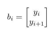
Taking all of these terms, we are able to solve for the H matrix in the following least squares equation!:

In order to solve for this, I simply used the np.linalg.lstsq function. Now we are ready to use the homography to warp our images!

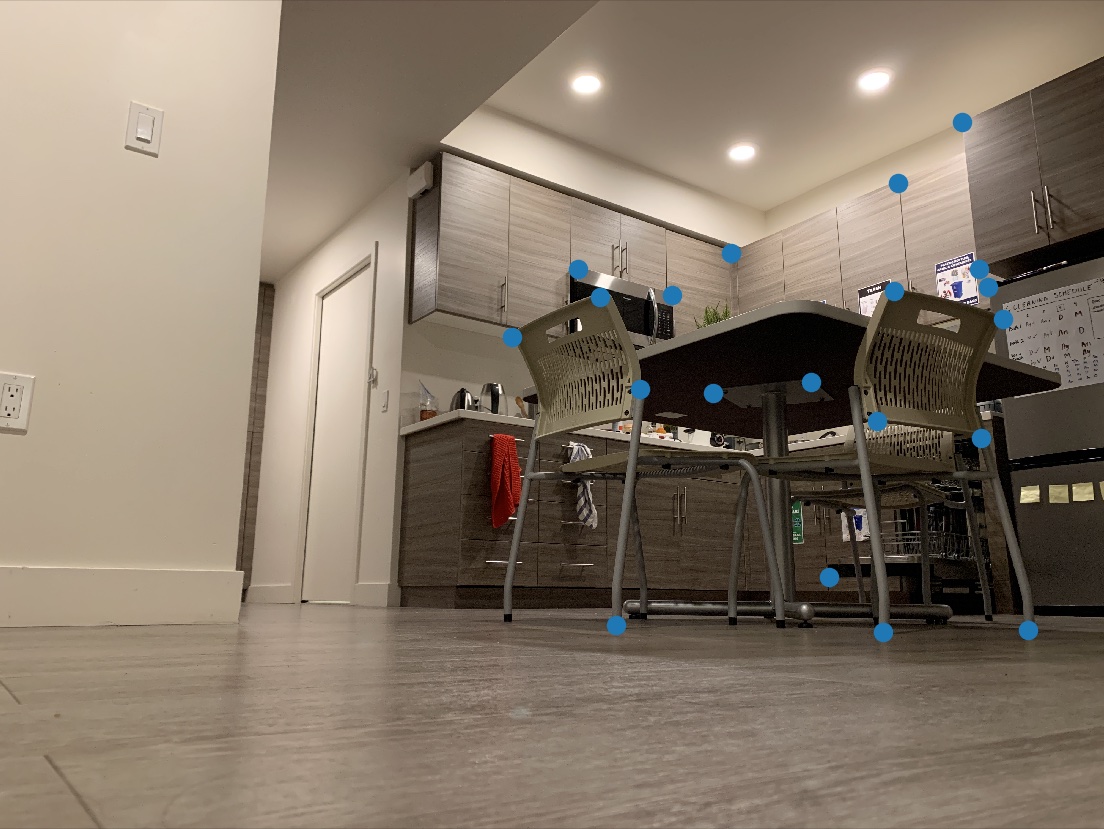
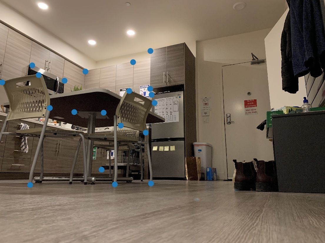
I tried to select around 20 keypoints. With any less than that, I found that the image came out blurry. I also found that if the keypoints were localized to a specific part of the image, it was more in focus at the region, but blurry in the regions where the keypoints were more sparse!

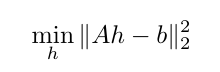
Warp the images

To warp the keypoints, I first found the homography matrix. Then, I defined the bounds of my warped image (to make sure that once it was warped, the final output still contained all of the colored pixels necessary and the image wasn't cut off). Then, I created a set of x and y indices for my original image, flattened these arrays, and multiplied them by the inverse homogenous matrix. This essentially creates an array of indices that represent where the original indices map to in the final, warped image. These are the computed input vectors that represent the x and y "target" / warped values, as compared to the original source image. After transforming these indices, we must normalize them in order to make sure they are still on the same scale as the original indices! We are then able to use the openCV remap function to compute the inverse interpolation for us, in order to find the ultiamtely warped image!

I was running into an issue where I'd warp the image just fine, but the image itself would get cut off. The solution to this was simply just to increase the width and height of the target image before using the cv2.remap function used to warp the image using bilinear interpolation, and this fixed the problem!

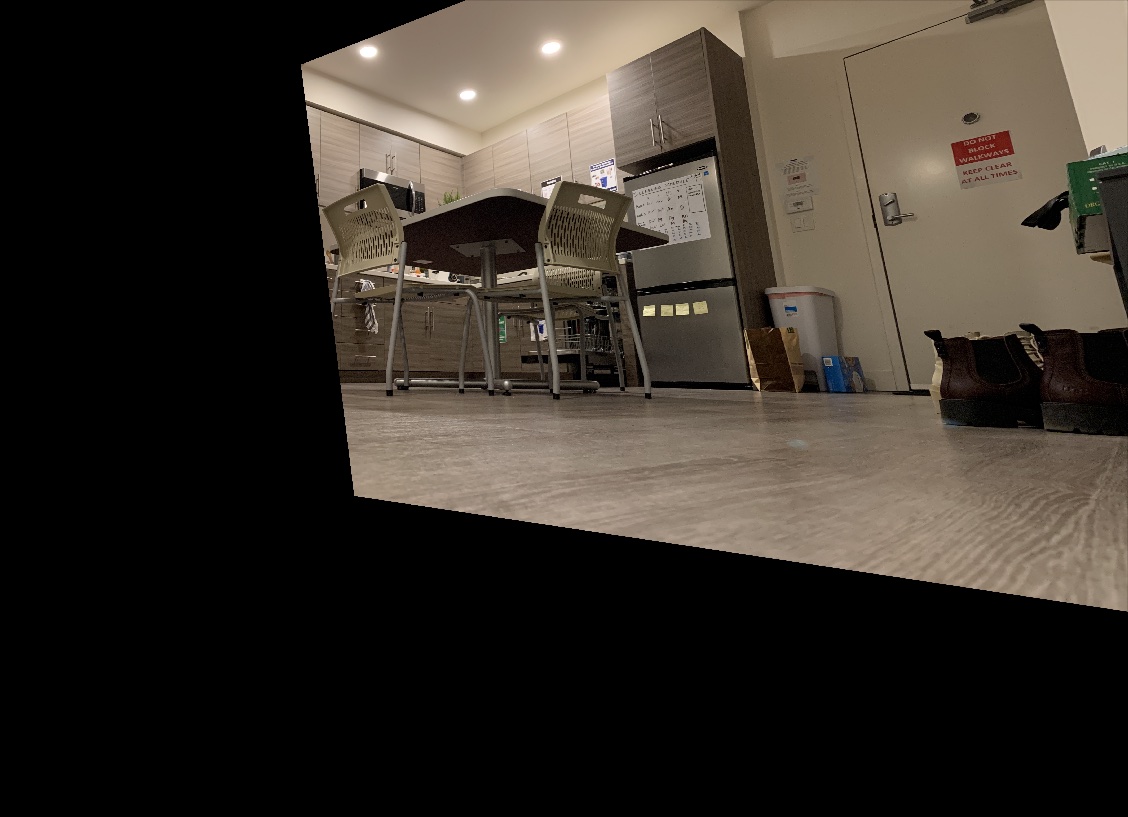
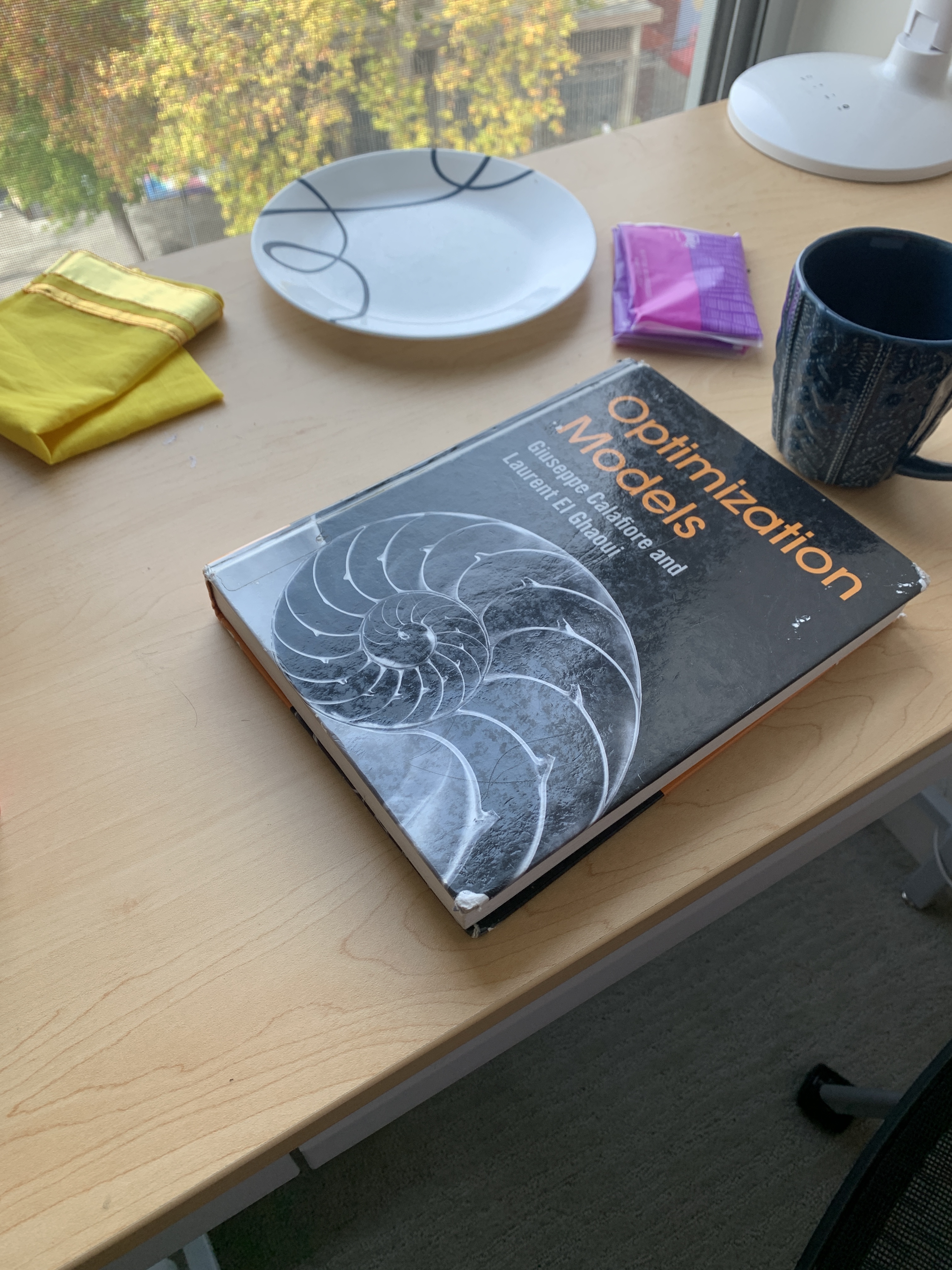
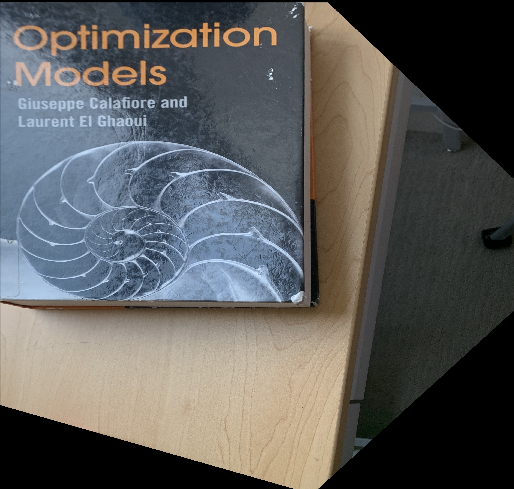
Image Rectification

Blend images into a mosaic

Finally, after creating our images, we can finally blend them together! The bulk of my logic for blending is contained in the layer_images function. I first alpha "feathered" both images. Since both of these images didn't have alpha channels, I manually added one (a channel of 1s). Then, I was able to For the left image, I linearly decreased the alpha value from 1.0 to 0.0, corresponding to the left and right sides of the image, respectively. I did this same sequence, but flipped, for the right images!

Then, since the warped image was resized to account for parts of the image falling out of the original image size, I also had to resize the non-warped image to be able to add them together accurately! In order to resize them, I simply padded the image vertically and horizontally with arrays of 0s to fill in the gap of the difference.

I noticed that if I added the points together at this stage, it wouldn't quite come out correctly because I would effectually end up averaging / normalizing parts of the image that were simply layered over arrays of 0s. As such, a way of combating this was to simply double the pixel values of the parts of the images that were not overlapping.

To do this, I replaced the zeros that were being added to the images with the pixel values of that part of the image, so when I normalized the whole image it ended up being the original / correct value for every part of the image!

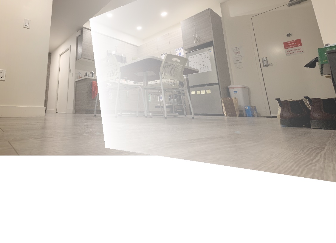
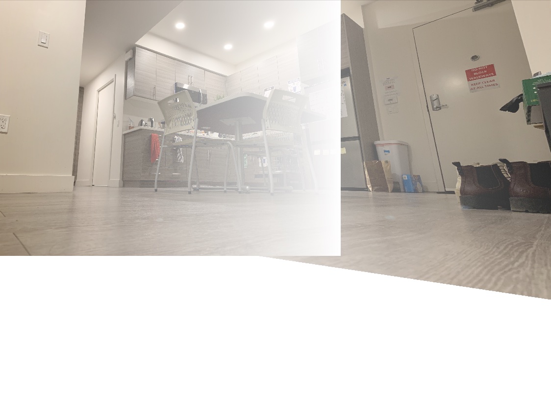
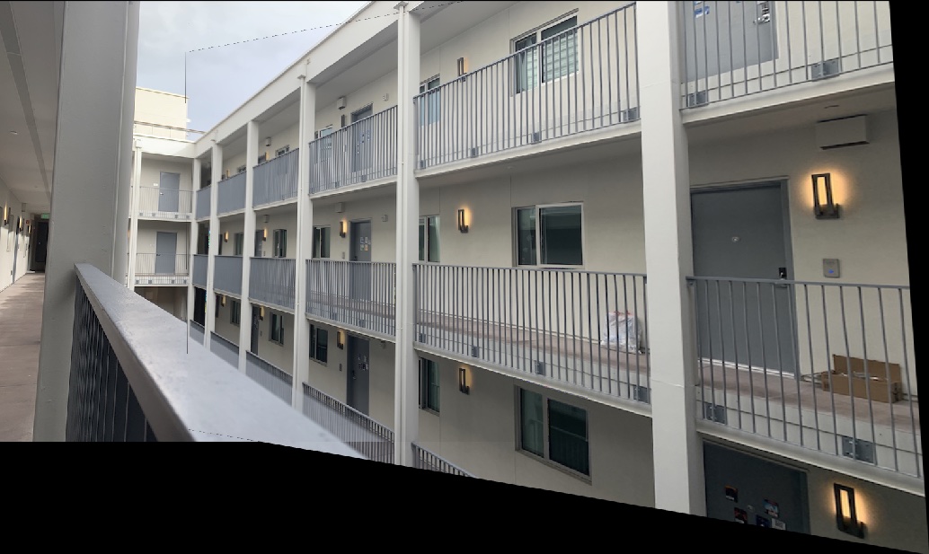
and here's the final stitching + some other examples!:

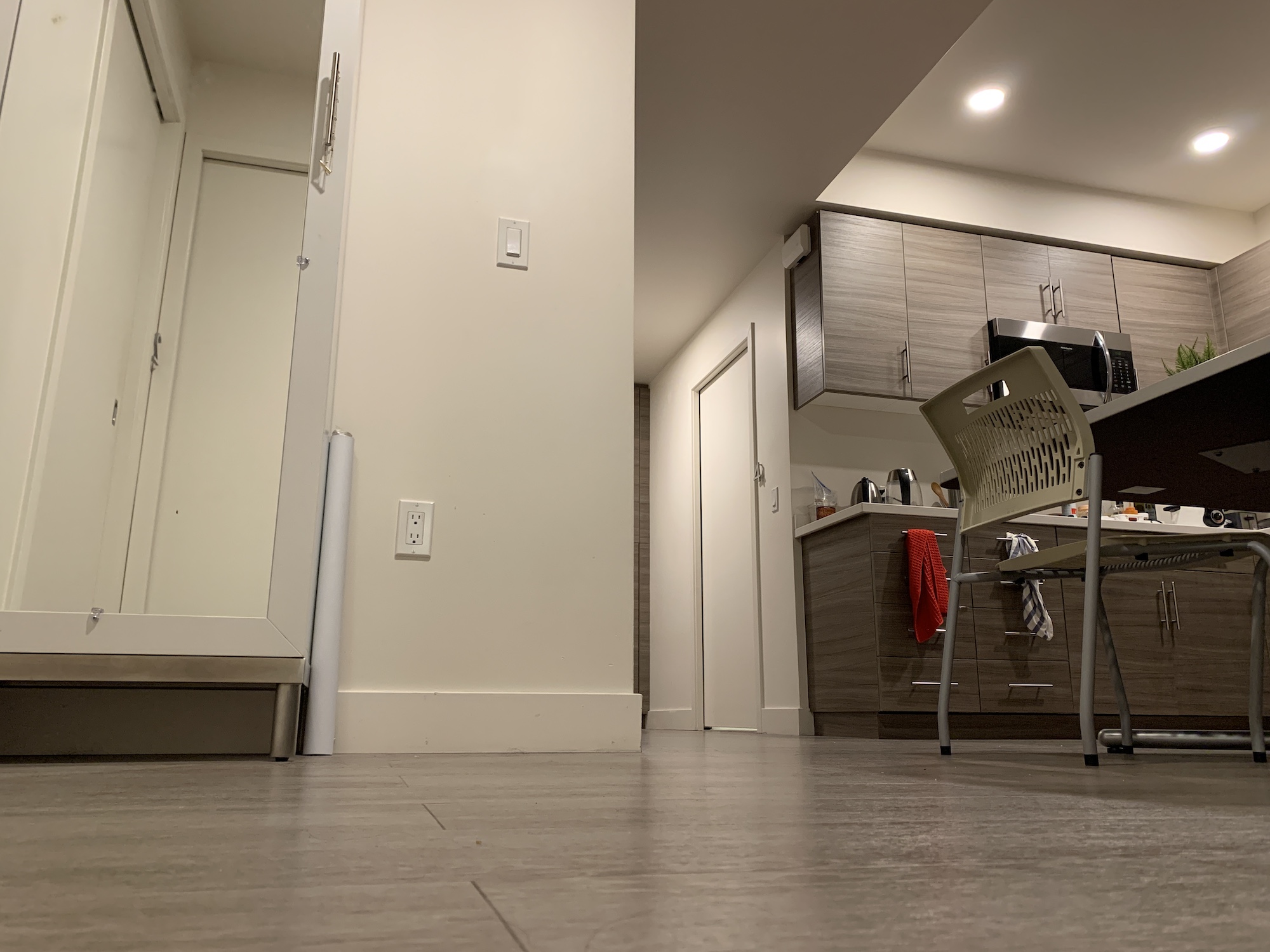
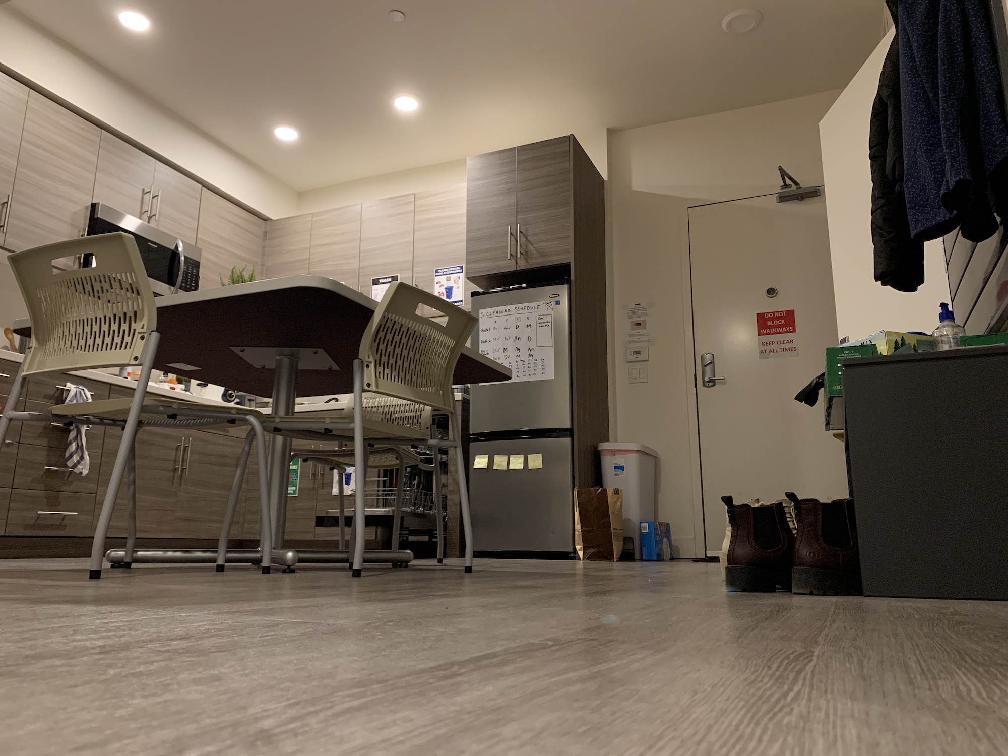
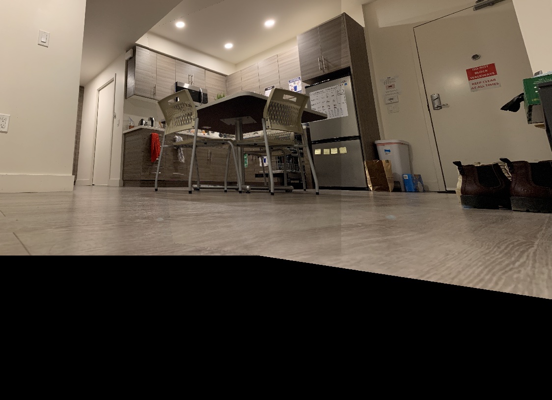
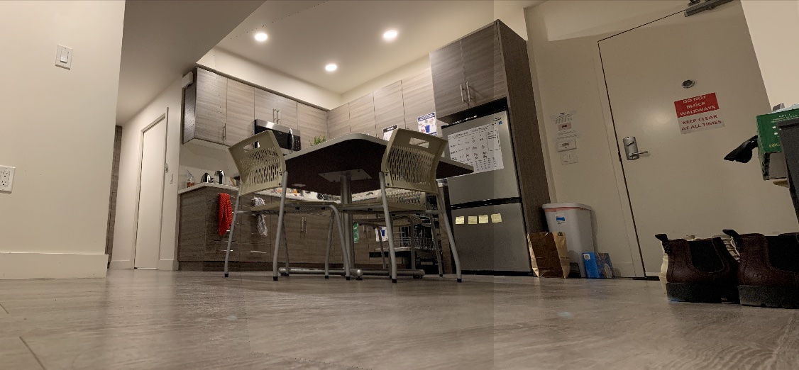
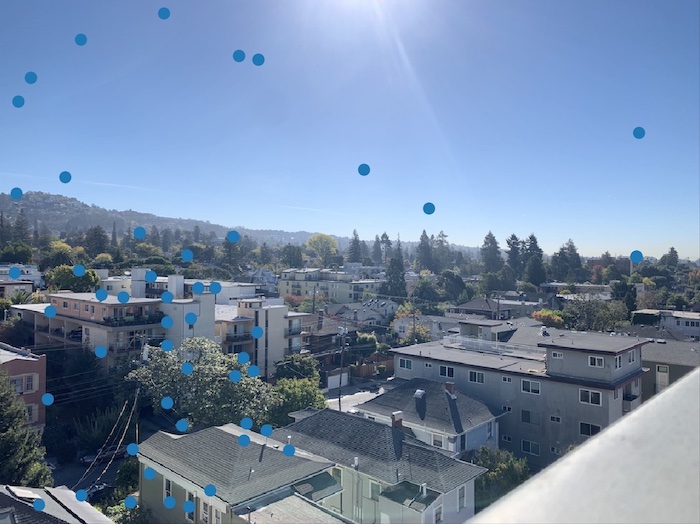
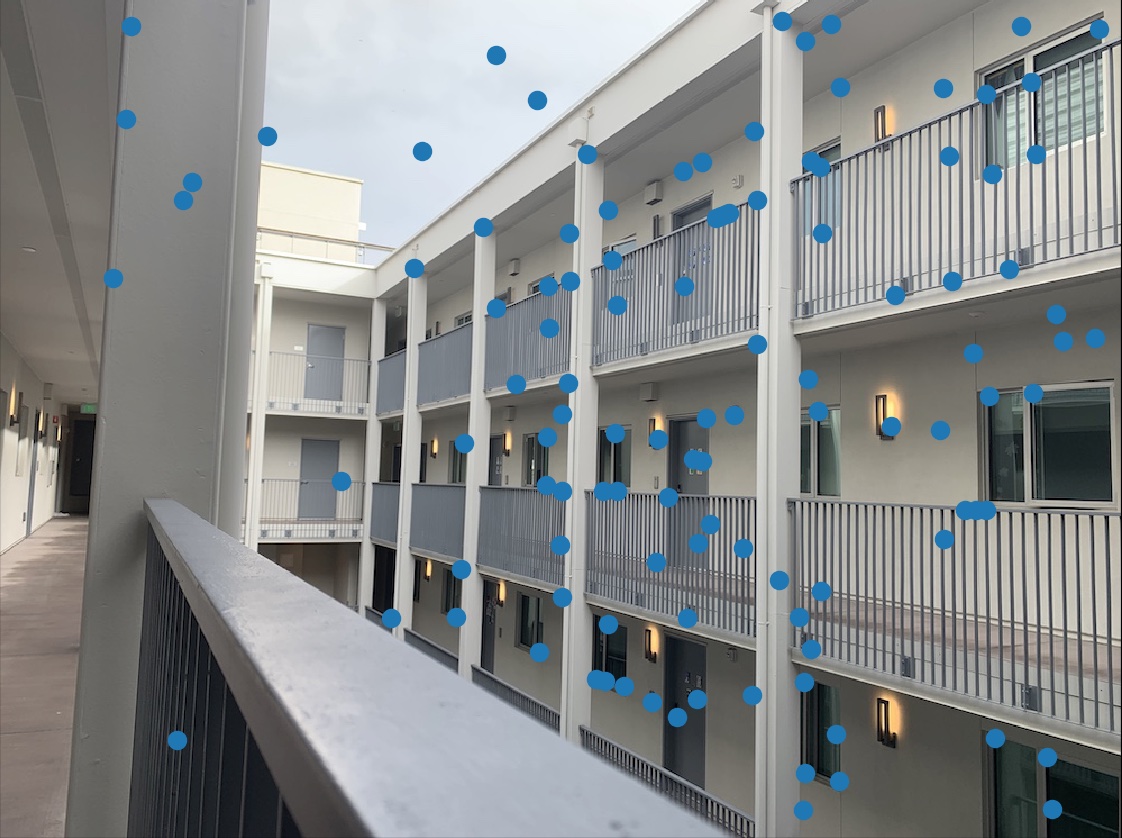
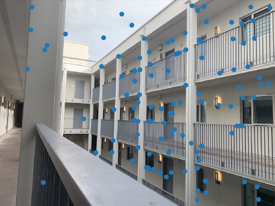
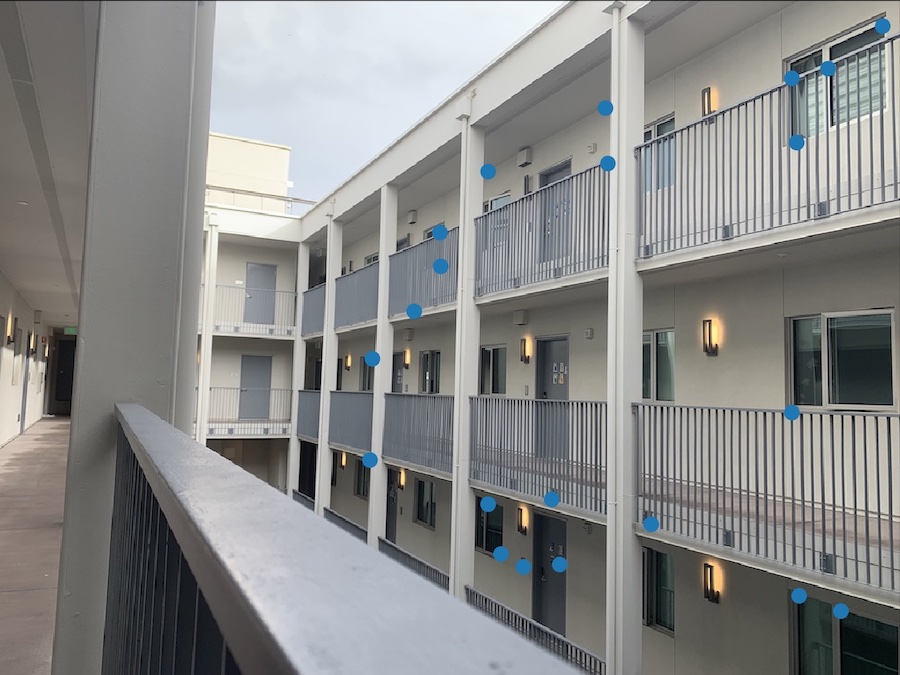
Image 1: "ants-eye-view" of my apartment aka a photo I took on my floor

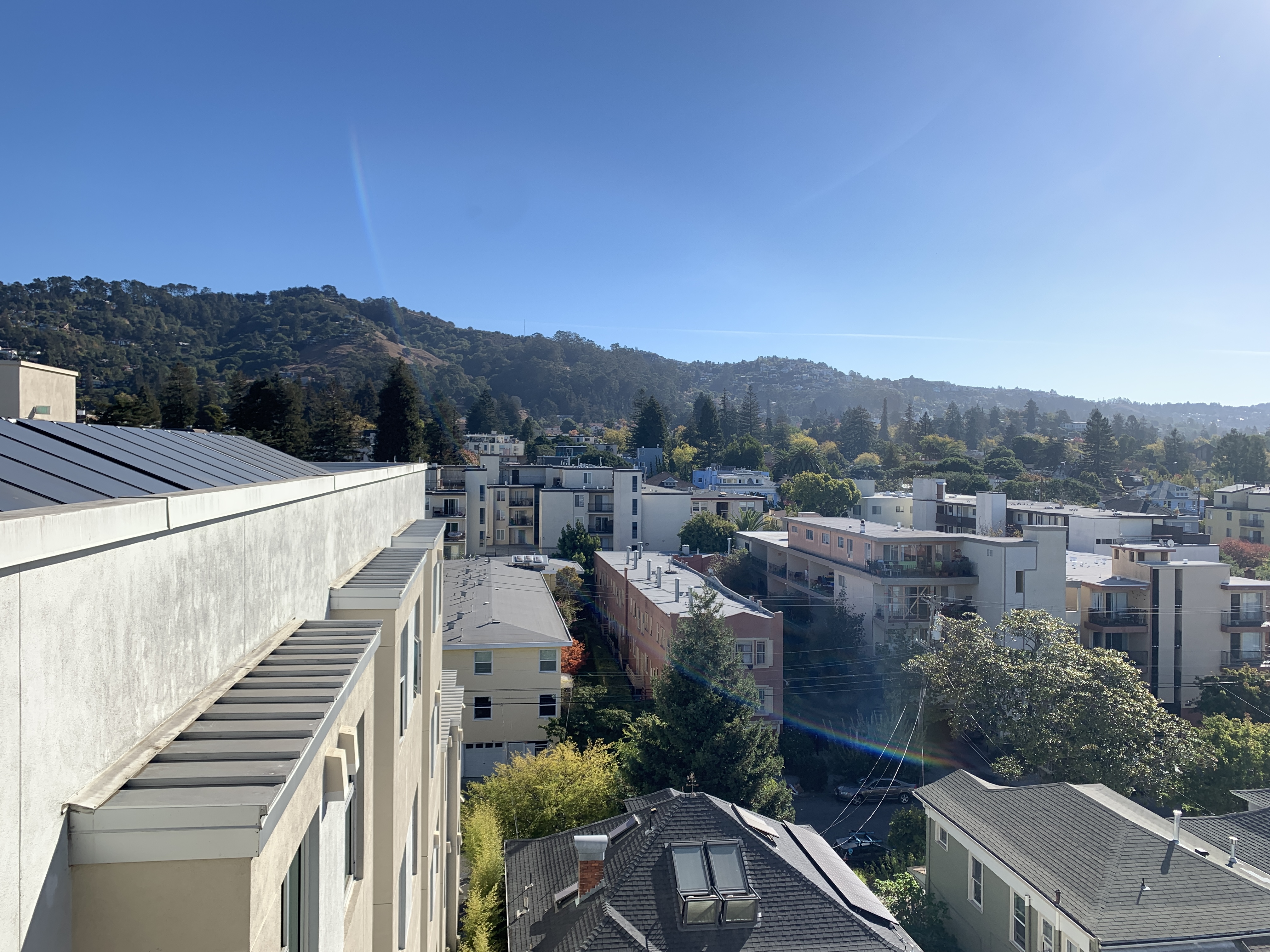
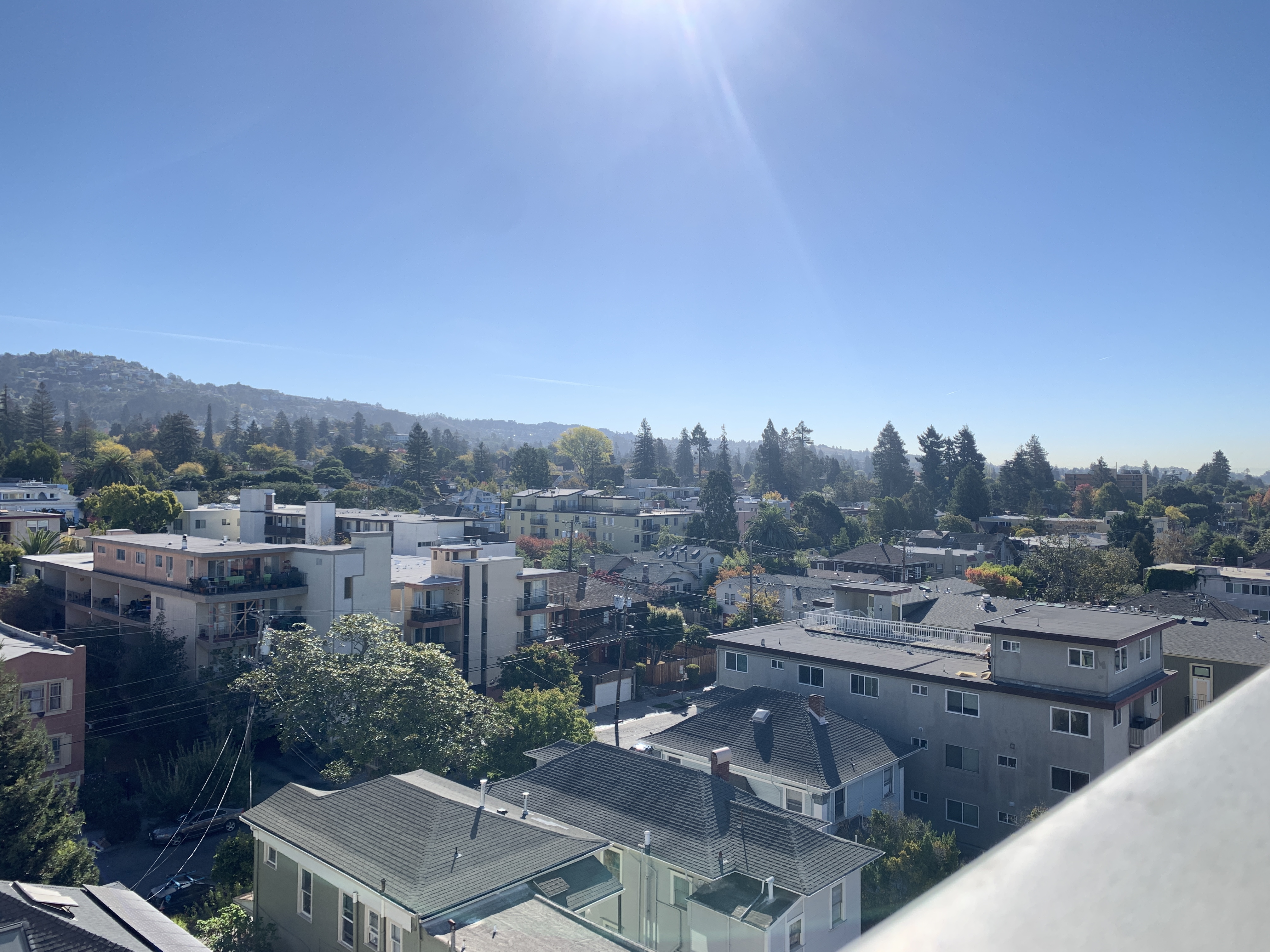
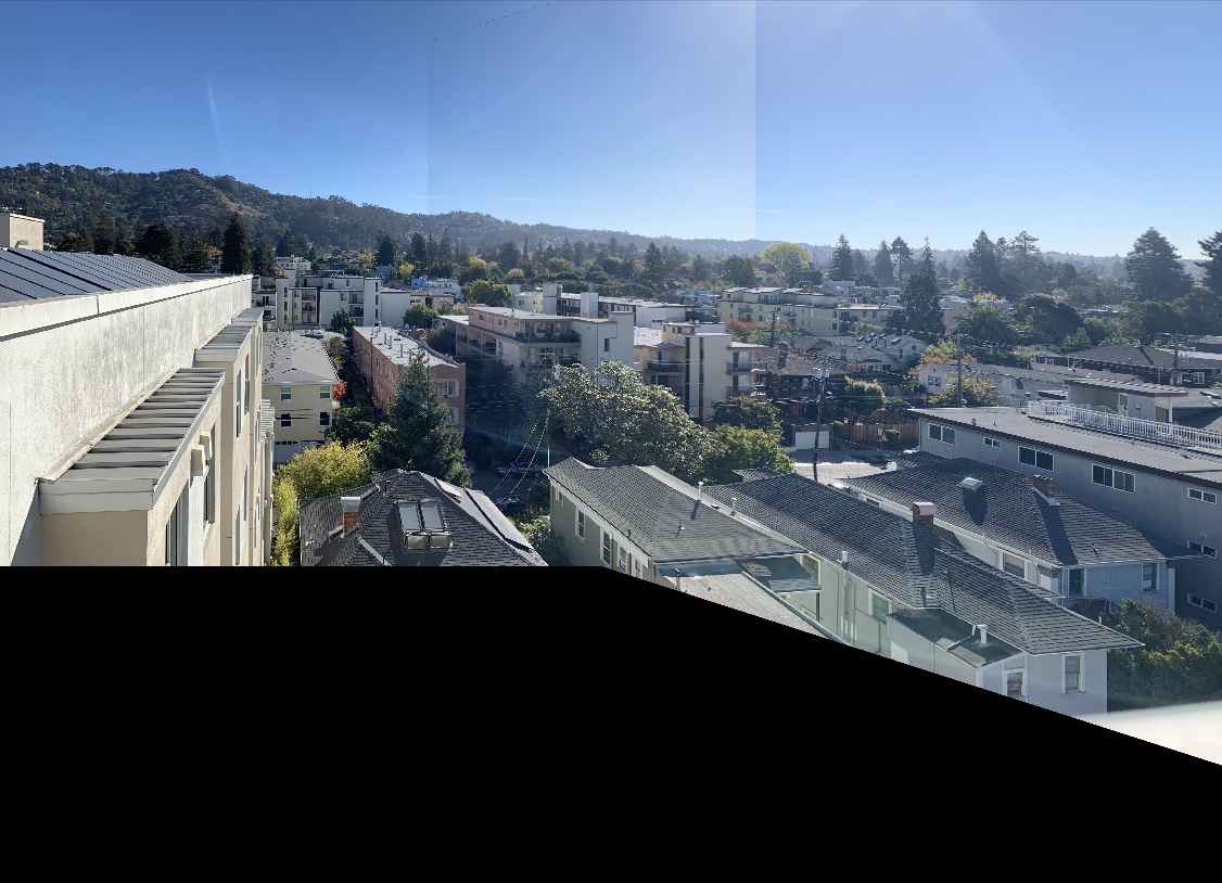
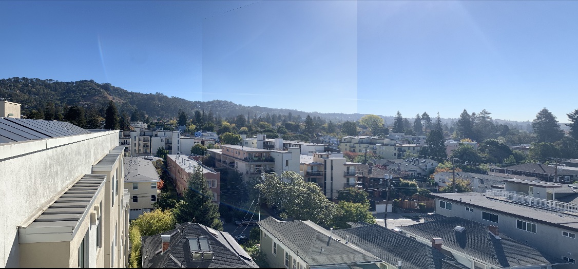
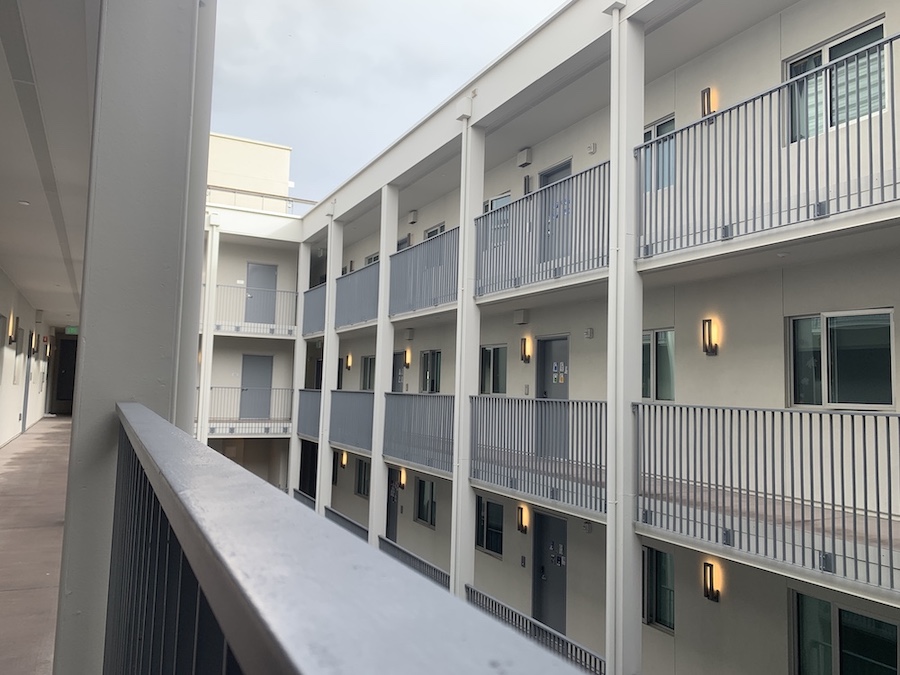
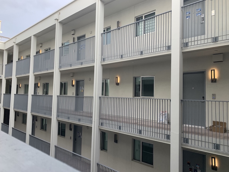
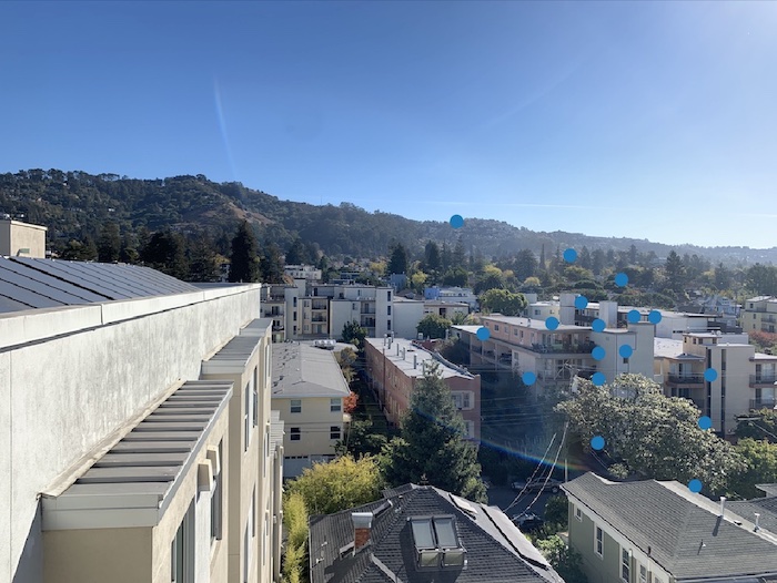
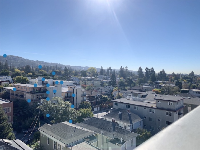
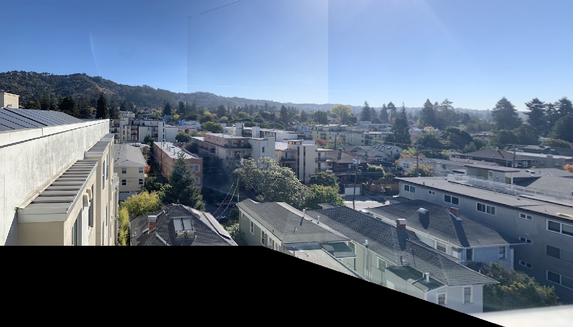
Image 2: Photo from my roof!

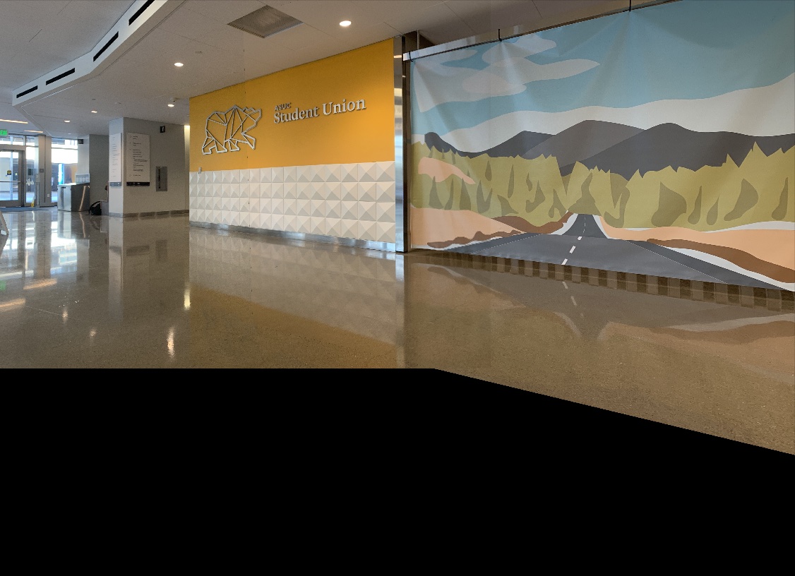
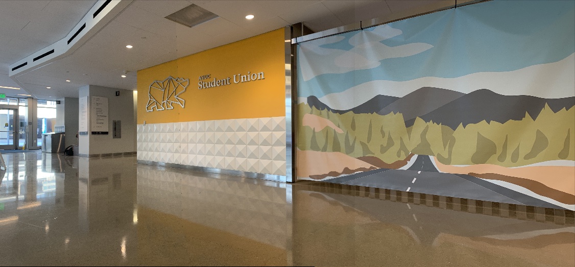
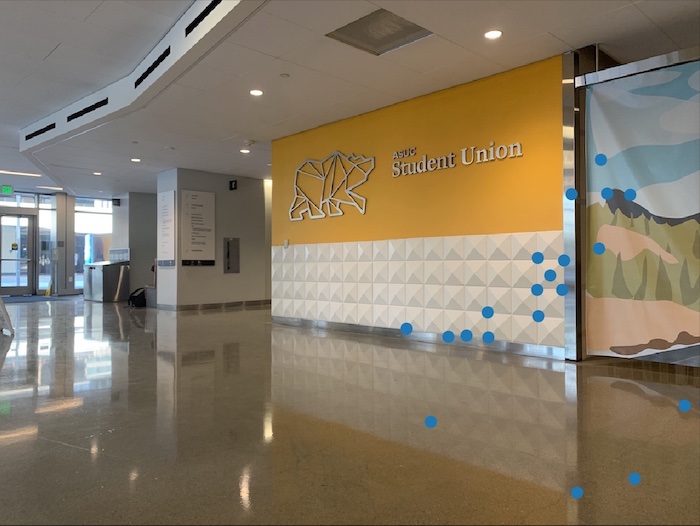
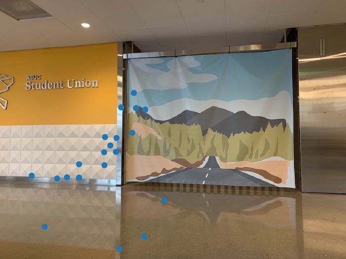
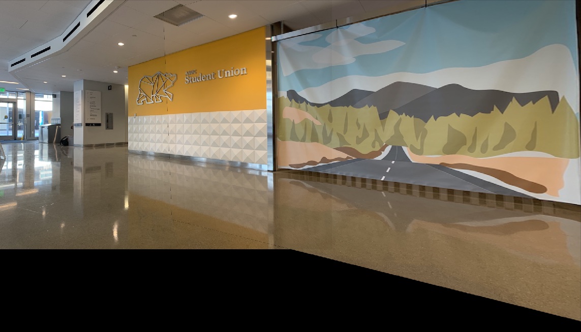
Image 3: Photo in MLK!

Coolest part of the project :)

The coolest part of the project is the fact that we had the ability to stitch together images using only a few points keypoints! I had always wondered how panorama stitching worked, so being able to both learn that in class and then implement it myself was super gratifying and interesting!

Part b: Feature Matching for Auto-Stitching

Overview

In the first part of this project, we created the panorama stitching algorithm that used manually-defined keypoints. However, in this part, we will be automatically finding keypoints in the image using corner detection and point / feature matching algorithms, allowing us to create (theoretically) cleaner and easier-to-create panoramas. The methodology detailed in the webpage follows from the paper "Multi-Image Matching using Multi-Scale Oriented Patches" by Brown, Szeliski, and Winder.

Staritng images:

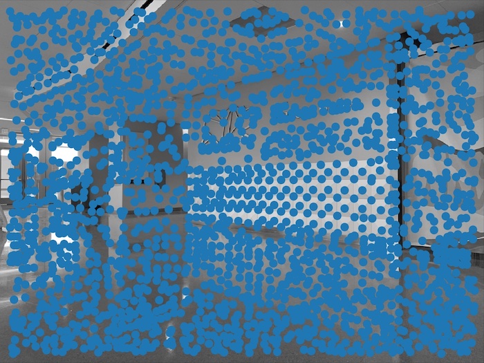
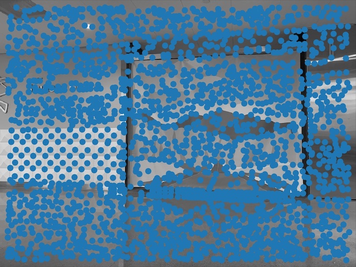
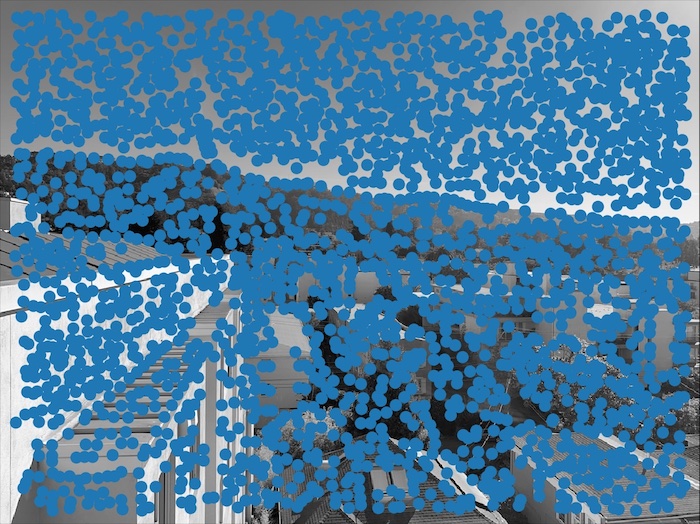
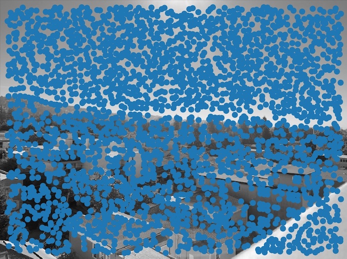
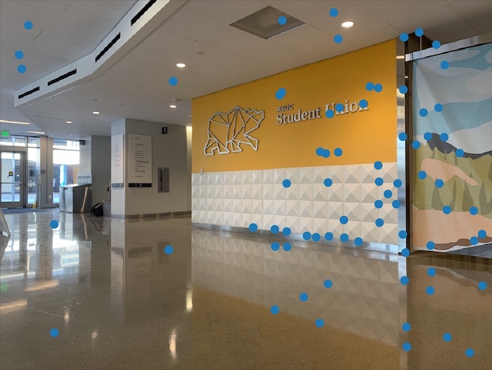
Detecting corner features in an image

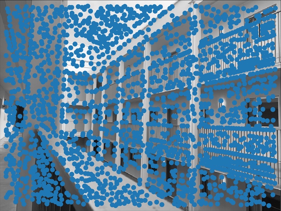
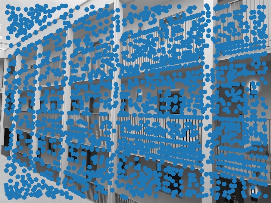
In order to detect corner features in an image, I used the Harris interest point detector algorithm to identify Harris points in the image. This was a function that was provided to us in the source code for the project. In order to calculate the adaptive non-maximal suppression (ANMS), I first calculated the interest points. This part pretty much directly followed the algorithm detailed in the paper! I looked at every combination of points within the calculated harris points and first checked if they satisfied the requirement that f(x_i) < c_robust * f(x_j), where f is the matrix of values that correspond to the harris corners' corner strengths , c_robust is a constant (that I have set to 0.9), and x_i and x_i are the corrdinates I am iterating over. In order to caluclate the desired interest points, we perform a form of robust optimization. So, for every coordinate, once I've gotten past the conditional statement, I first initialize the radius to be the largest possible value, infinity. Then, I find the smallest distance between this point and another point in the harris matrix (where distance is defined by an L2 norm). The smallest distance found is the given "radius" for the point. I then constructed an array of all of the radii and points. Ultimately, I want the points that have the largest radius because that implied they carry the most weight. Therefore, I sorted my array by the radius values and simply used the top 500 values from that list -- these are the values / interest points that carry the most "weight" in the value because it maximizes the minimum of the distance between each strong point. Therefore, it is most likely to be good corners to use for further computation! Because the harris corners algorithm detects many points, it can be difficult not only to view, but took a long time to process a single image. Therefore, to optimize this process, I simply downsized my image and increased the sigma value to 3 in the harris corners function provided to us, which greatly reduced processing time for ANMS!

Harris points:

Interest points from ANMS:

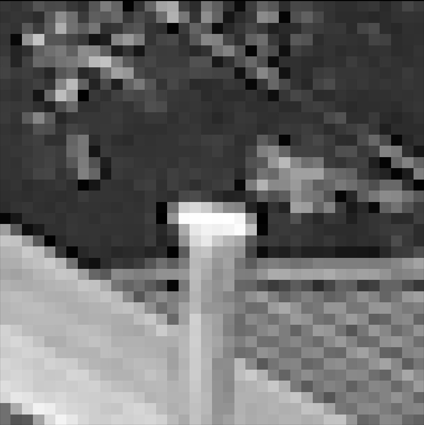
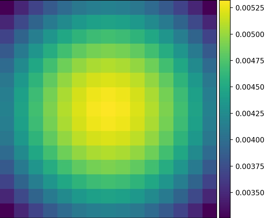
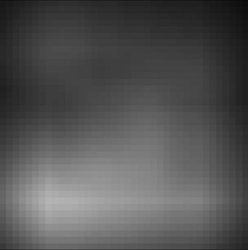
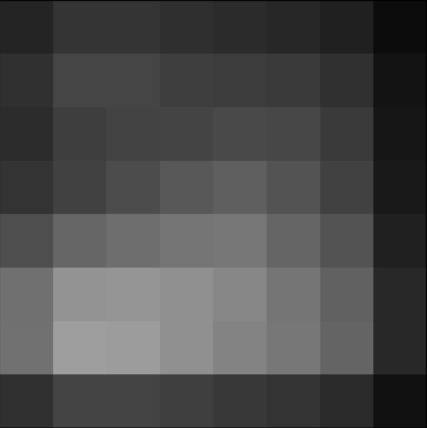
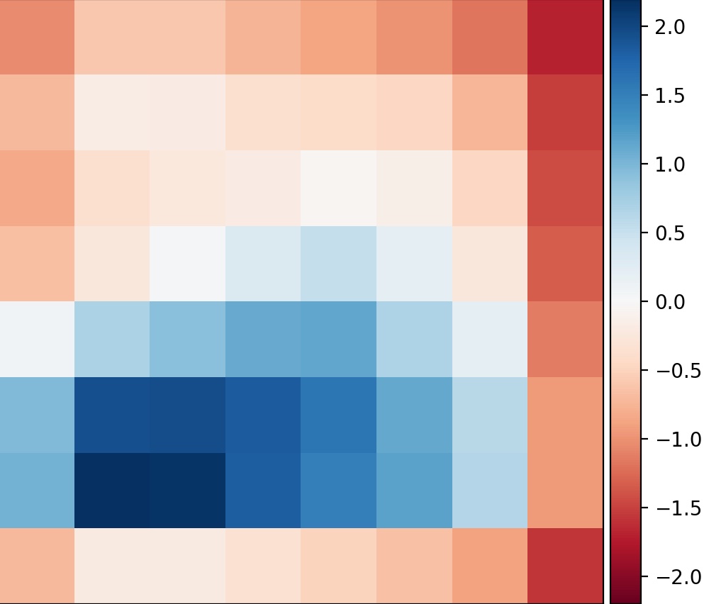
Extracting a Feature Descriptor for each feature point

In order to extract a feature descriptor given the interest points, the general flow is to extract a patch, convolve it with a Gaussian, downsize it, and continue. We must first filter and downsample our patch in order to remove high frequencies in the patch. This is important because the features we are looking at features in both images, with the ultimate goal of matching them. In order to find similar images, we want to find feature points that exist on large landmarks in the image (like corners) rather than the small details that can lead to misalignments if matched. After downsizing and blurring our image, we normalize it in order to make the mean 0 and the standard deviation 1, which serves to make the images more invariant to bias and gain!

Example feature descriptor processing:

Matching these feature descriptors between two images

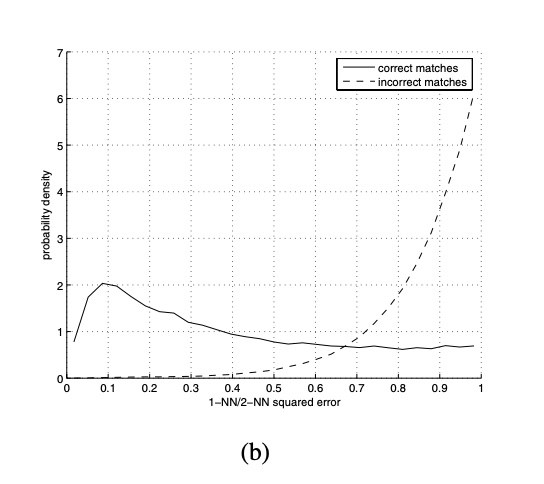
Once we have computed the feature descriptors, it is then possible to match the points. Essentially, I calculated nearest neighbors between the two images, on each of their features points. This allowed me to compute the "closest" points to one another, and therefore, the "nearest neighbors". Taking these neighbors, I calculated the error between its point and the point we are comparing it to (e_nn1, e_nn2). According to Lowe, we are able to use the ratio of these two errors (e_nn1 / e_nn2) to match features with a well-separated distribution. I picked the value of 0.66 as my epsilon threshold, but by making that number lower it is possible to get values with less and less error!

Consulted this figure in the paper to determine my threshold of 0.66:

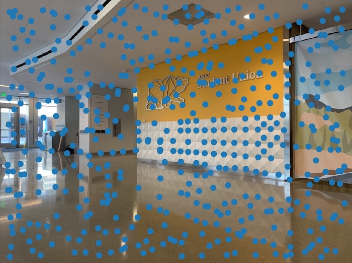
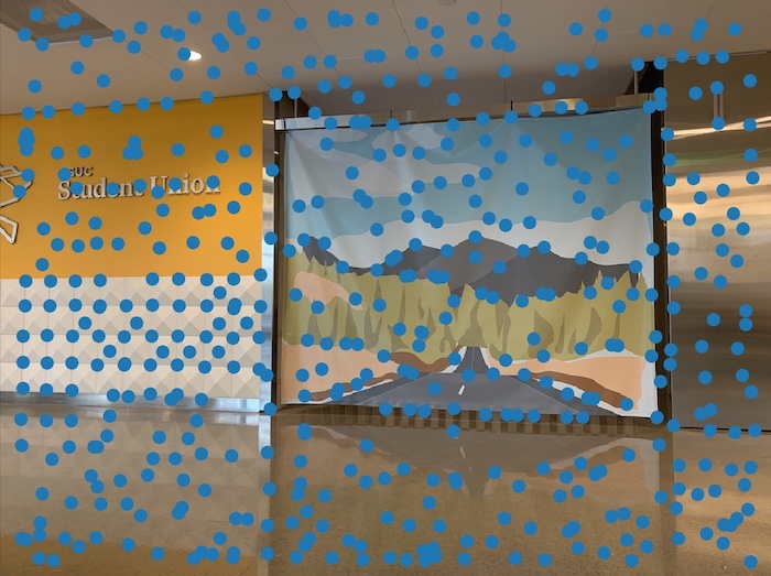
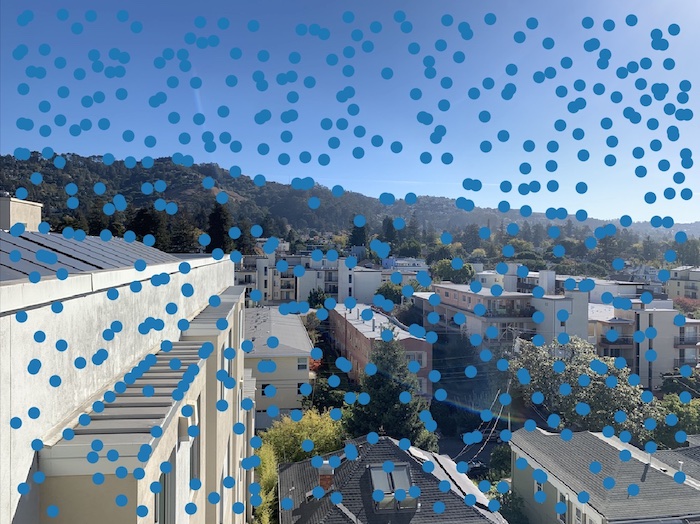
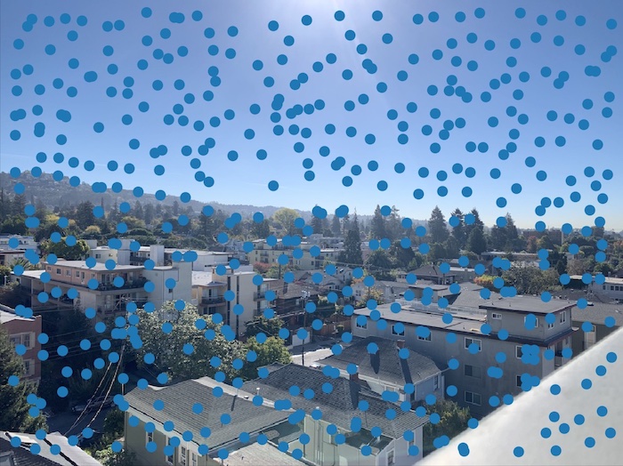
Points after running feature matching algorithm:

Use a robust method (RANSAC) to compute a homography

Finally, I ran the RANSAC algorithm to compute the final homography matrix. In this algorithm, I ran a loop where I selected 4 feature pairs, computed a homography based on those pairs, and then computer inliners in which the L2 distance between the warped points (initial points of an image multiplied by the homography matrix) and the destination points of the other image are less than an epsilon threshold. I repeated this process 5000, saving the largest set of inliner points as my "final" set of inliners! Using my final, most optimal inliner points, I recomputed the homography matrix for the final homography. After this, I was simply able to rerun my algorithm detailed in part A for warping, combining, and blending the images to create my homography!

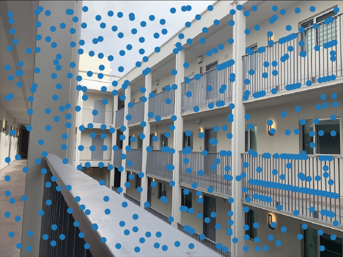
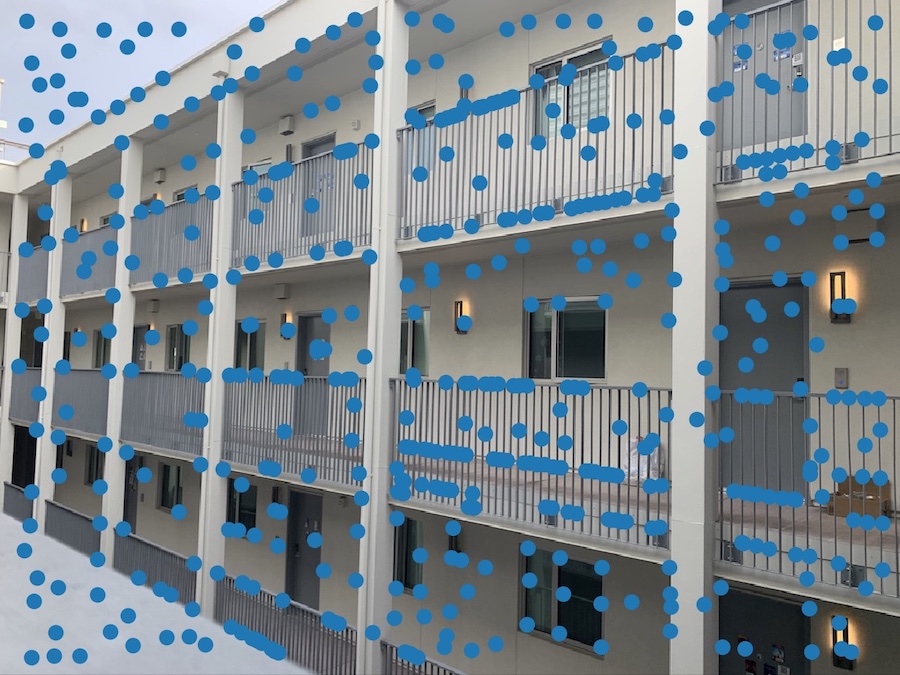
Points after running RANSAC algorithm (all points on each image have a corresponding point in the other image!):

Mosaics

Final panoramas!

Cooolest part of the project :)

The coolest part of this was the feature matching process. It was really interesting to see how we were able to take two similar, yet differently oriented images and not only detect keypoints on the image, but actually match them to one another! Especially after having spent so long picking my own points for these panoramas, it's incredible to see just how much faster it is to programatically create stitch these image together!