Overview

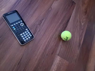
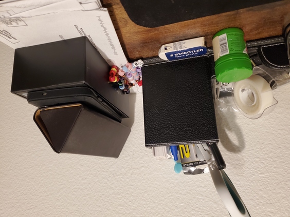
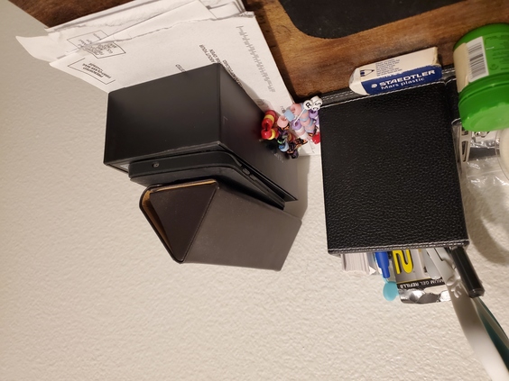
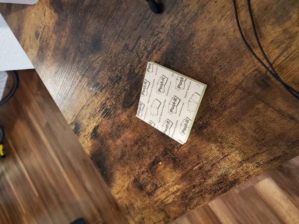
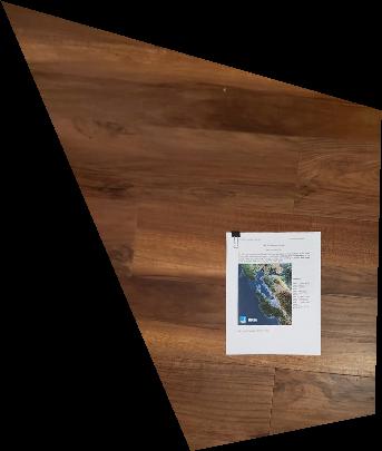
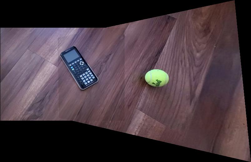
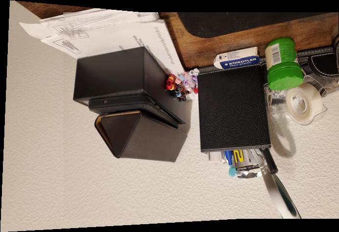
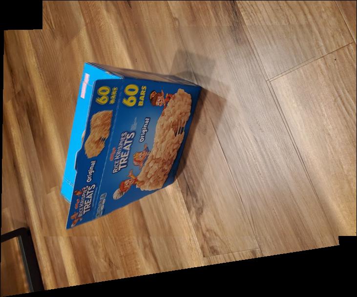
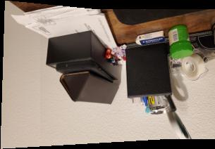
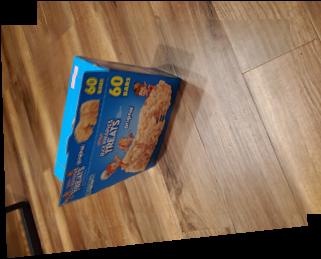
If we use a camera take a picture of the same scene in the same position from a different angle, we can estimate the transformation between the two images as a perspective projection. Determining this transformation matrix H will allow us to merge the images into a single mosaiced image. I shot several images at different angles. These images are shown below.

Recover Homographies

Similar to project 3, in order to get a good result, correspondences (keypoints) must be defined first. To find the transform matrix H, we can unroll the matrix into a column vector h. From here, we can expand the relationship H*v = v', or [[a b c] [d e f] [g h 1]] * [[x0] [y0] [1]] = w * [[x1] [y1] [1]] where w is some arbitrary scaling vector. Expanding this out in terms of H's contents will allow us to find two systems of equations for the variables inside of H (one for each coordinate, x and y). Thus, given four coordinate pairs we can uniquely determine all contents of h. We write this as Ah = b, where A is an 8x8 matrix and b is the an 8x1 matrix consisting of the four points' column vectors stacked on top of each other.

A perspective projection transform is uniquely determined by four pairwise corresponding points, but this would be highly susceptible to noise. To protect against noise, we can overdetermine the system by selecting more than four points. We can then use least squares to determine the closest fitting h, by simply doing inv(A^T * A) * A^T * b.

Warp the Images

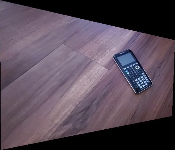
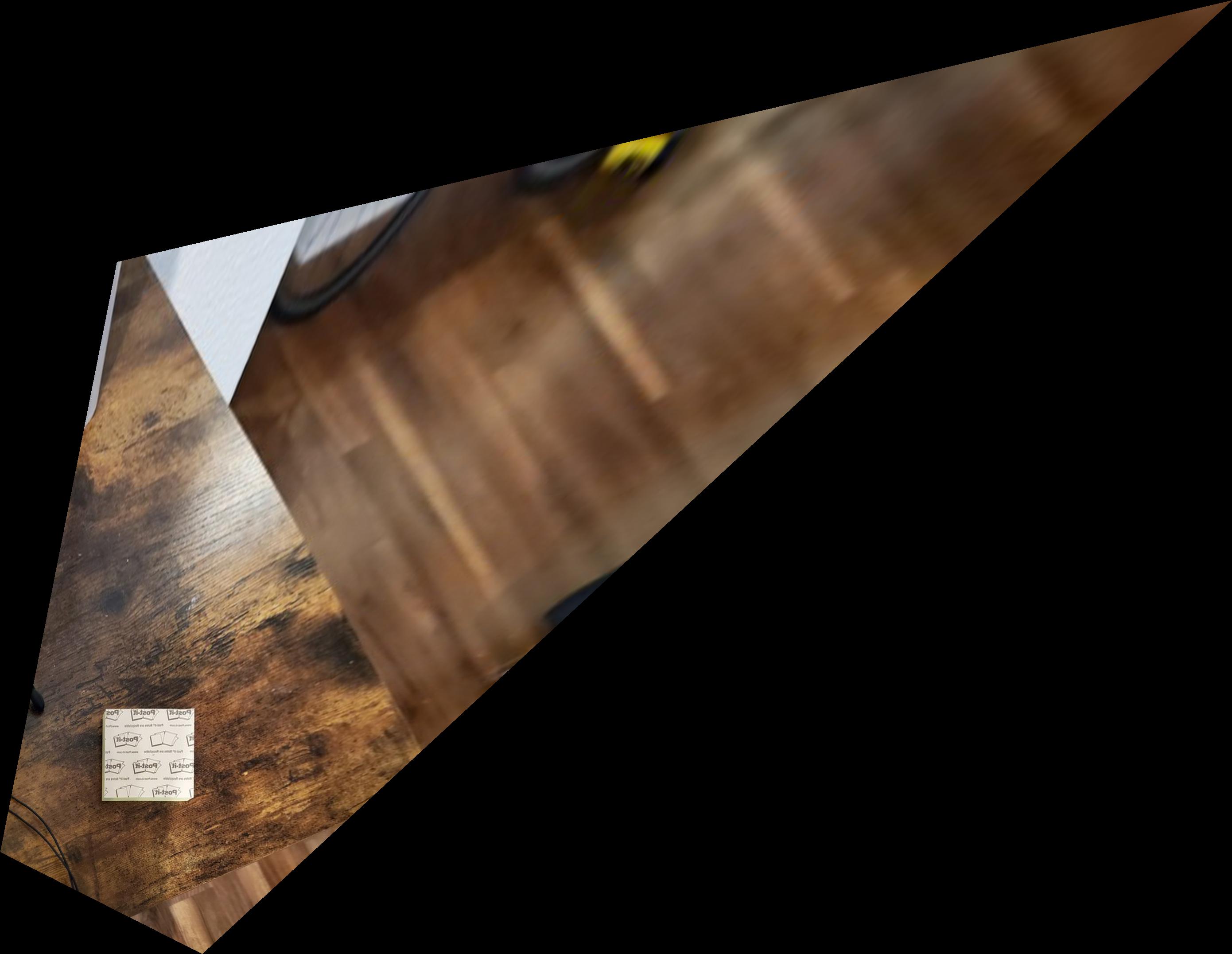
Provided the perspective transform, we can warp images to match each other. I used an inverse warp; for each pixel inside my final image, I multiplied the coordinate by the inverse of the homography matrix to determine which pixel in the original image the current value should correspond to, and interpolated if the pixel index was off an integer value. A calculator is shown at two different angles below; one angle is then warped to match the other.

We can also rectify images, such that square or rectangular items viewed from an angle get projected into a normal shape.

Blend Images Into a Mosaic

Given two identically warped images, we can overlay the matching parts to create an extended version of the original images. I did this by creating a blank canvas, and adding images onto it. I applied a mask that was 1 everywhere except for where image 1 and image 2 were both non-zero, where I blended the overlapping area together to create the final image. The products of this method are shown below.

Detecting Features

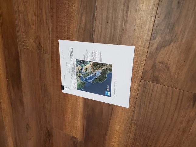
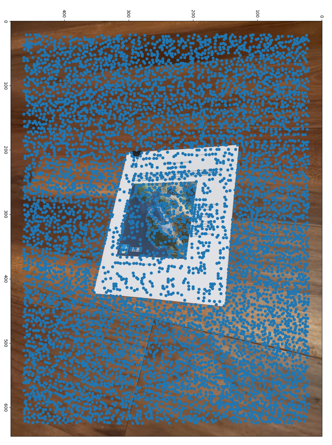
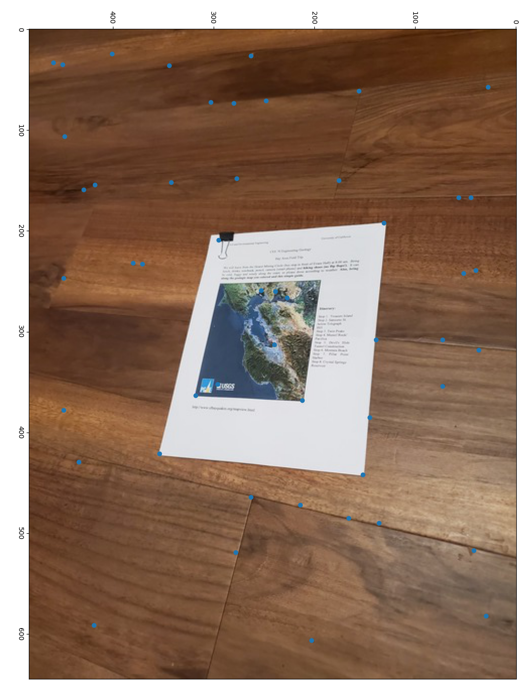
Harris corner detection uses gradients to detect corners of interest. I used the provided code to return the coordinates of these interest points, as well as the corner strength h of each individual pixel. Below is the output of the corner detection function after being run on a picture of paper on the floor.

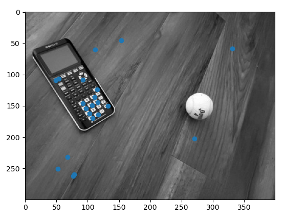
Adapative Non-maximal Suppression

Identifying corners of interest is useful, but not that great at detecting a quality sample of features that can help us determine correspondences between two images. As seen from the image above, we end up getting a lot of "points of interest" that actually are not very interesting at all. We thus need a way to get only the most interesting points, while also making sure that these points are spatially well-distributed; otherwise, if we simply took the largest absolute corner strengths in the image, we could potentially end up with only points located in an area with many strong corners, which would not necessarily overlap areas with a second image we wish to find correspondences with.

We thus implement a feature that finds the n most prominent localized points of interest - that is, n points of interest that are larger than all other points of interest around it in a radius r, for the largest possible r. We achieve this by first determining the globally maximal point of interest. We then set a radius of suppression for each interest point, which is the radius around the interest point where 90% of the strength of all points around it are no more than the strength of the interest point. The suppression radius for all interest points is initialized to be the distance to the global maximum, then we iterate through points and reduce the suppression radius as we encounter points that have sufficiently greater strength. We then sort each point by its radius of suppression (the globally maximum point has an infinite radius), and choose the top n points to remain. The results of this algorithm are shown below. Notice that the points of interest are now well-distributed.

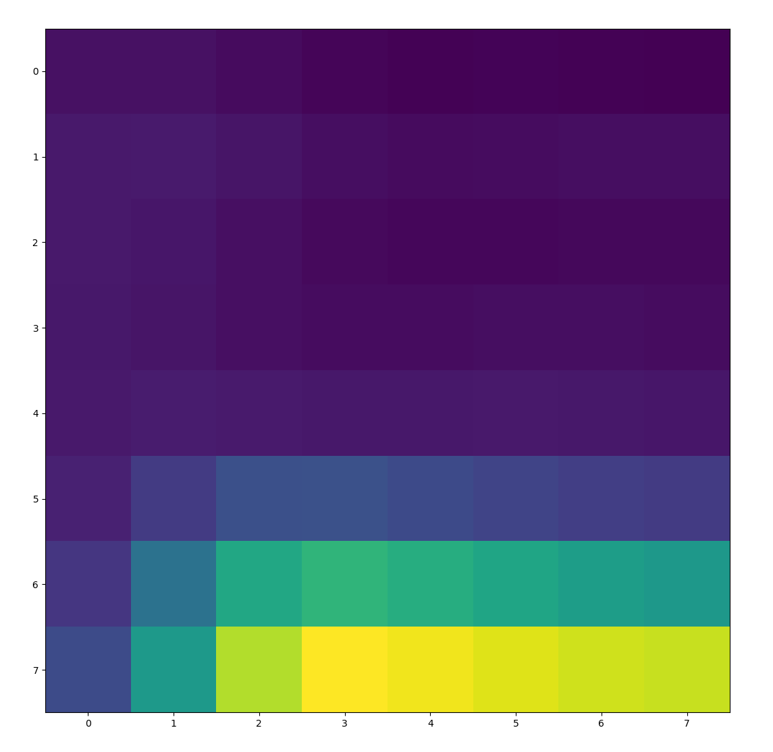
Feature Extraction

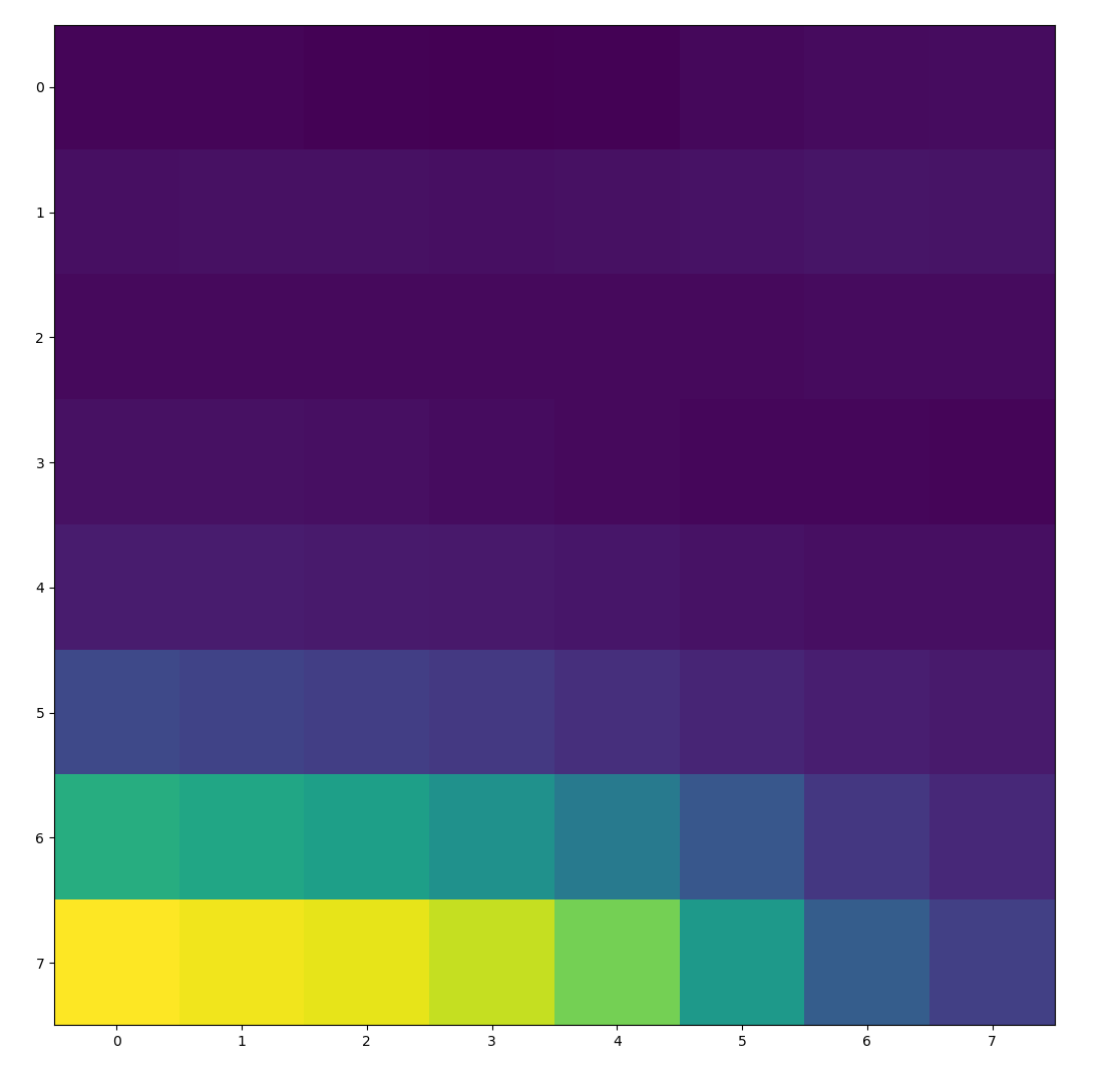
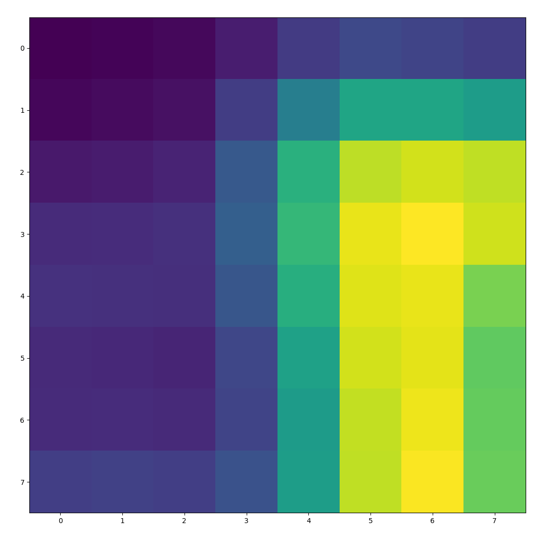
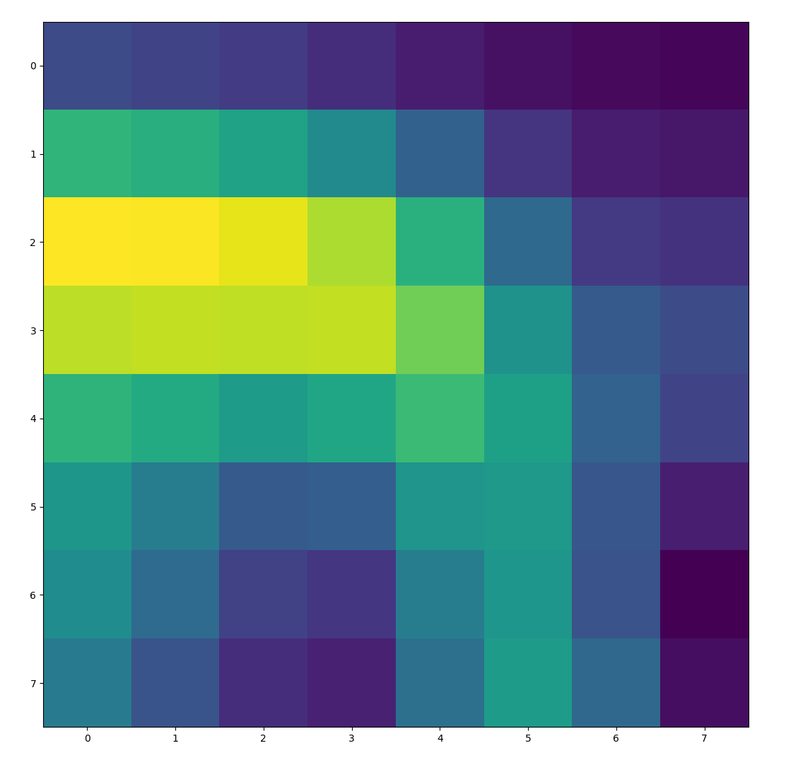
To extract features, we first low-pass filter the image by putting it through a Gaussian blur. We then sample a 40x40 window around each point of interest, and downscale to an 8x8 feature. This 8x8 feature is also normalized to have a mean of 0 and variance of 1. The blurring is done for antialiasing purposes. The images below show a few features that were extracted from the paper image above using this method.

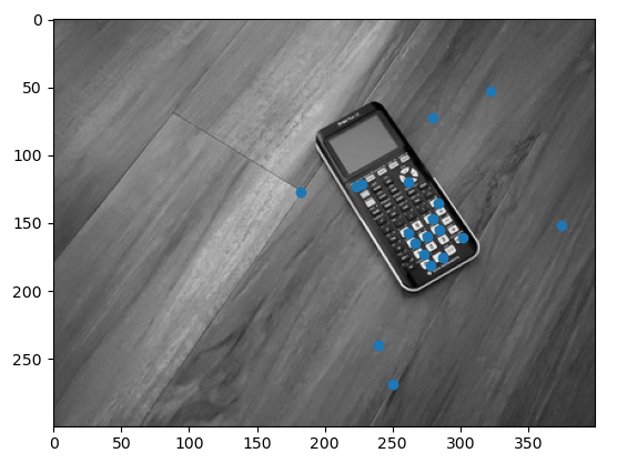
Feature Matching

Now that we can extract features and descriptors from an image, we can do so with a second image, and thus will have two lists of features. We can then compare these two lists to see which features align with one another. My method of comparison was the sum of squared differences (SSD), where we sum the square of pixel-wise differences between the two features. We compare each feature from one image to every feature in the other image, and look at the feature pair with a minimal SSD. In order to make sure we get good matches rather than something that happens to align due to noise or coincidence, I additionally compare the minimal SSD to the second minimal SSD, and only accept the feature-point pair if the second minimal SSD is more than twice as big as the minimal SSD. The results of running this on a pair of images is shown below.

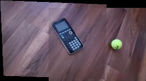
RANSAC and auto-mosaicing

As we can see from the images above, identified points of interest can be quite noisy. We thus need a way to identify the good points that can be used to calculate a homography. For this, I used the RANSAC algorithm, which randomly takes 4 points for a homography and continuously tests potential homographic transformations until we find one that aligns the best with our actual data points. This is determined the number of 'inliers', or points that fall within some acceptable error margin after being put under the test transformation. From there, we simply use the same algorithm we used in past parts to mosaic the images together. Results are shown below, with auto-aligned on the left and manual on the right. Note that the auto-aligned images were resolution reduced to save time.

What I've Learned

I've learned that transform matrices give us a lot of information! (not just perspective projections). Once a transform matrix is determined we can do a lot of things with it that are visually very interesting. Also, dealing with noise is a tricky problem! RANSAC is a pretty cool tool to deal with it.