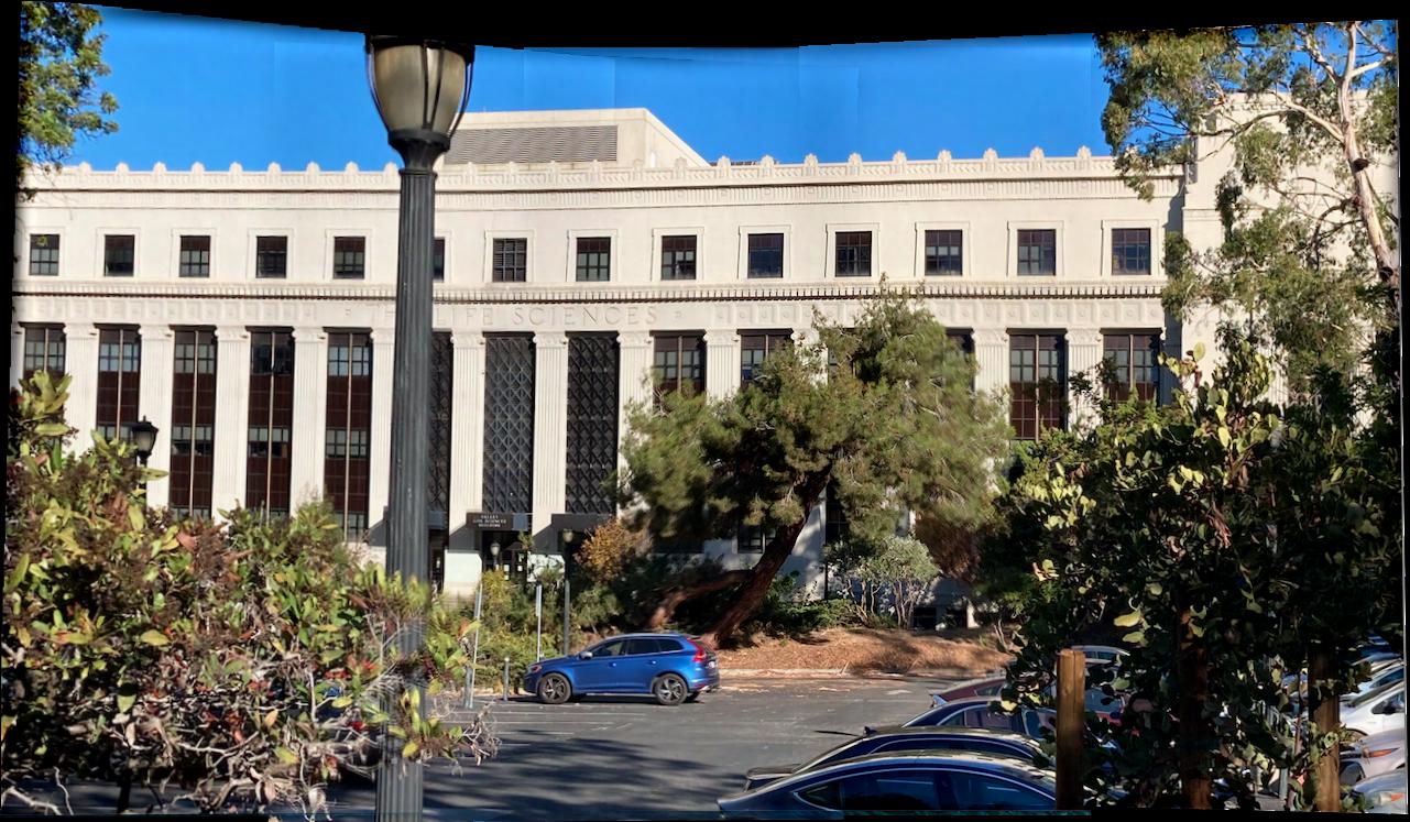
Overall one thing I thought I was pretty cool was how well we could blend together the different images to really make it feel like it came from a single capture. Granted some of the mosaics are better than others, but I felt I wasn't extremely careful taking photos making sure the camera didn't move so thought it was pretty cool that it came out as well as it did.
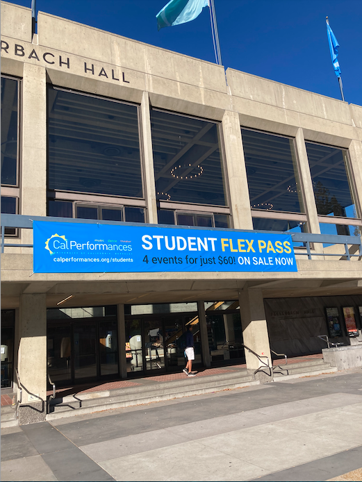
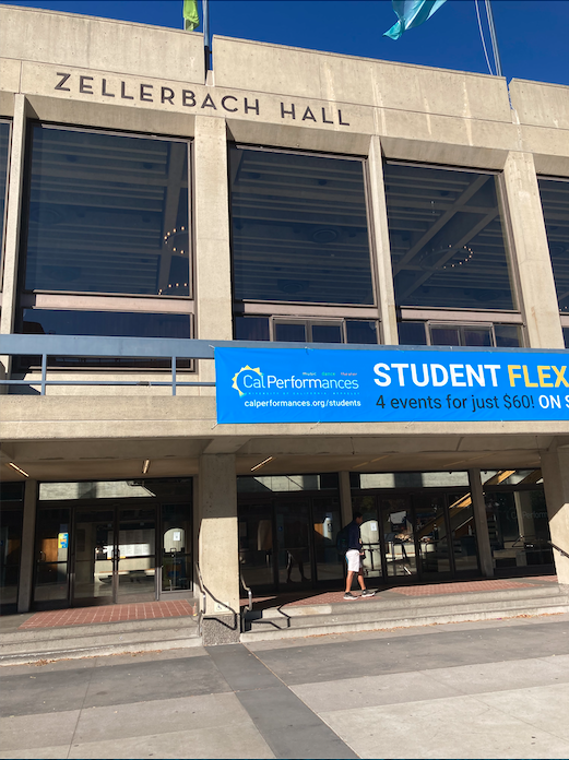
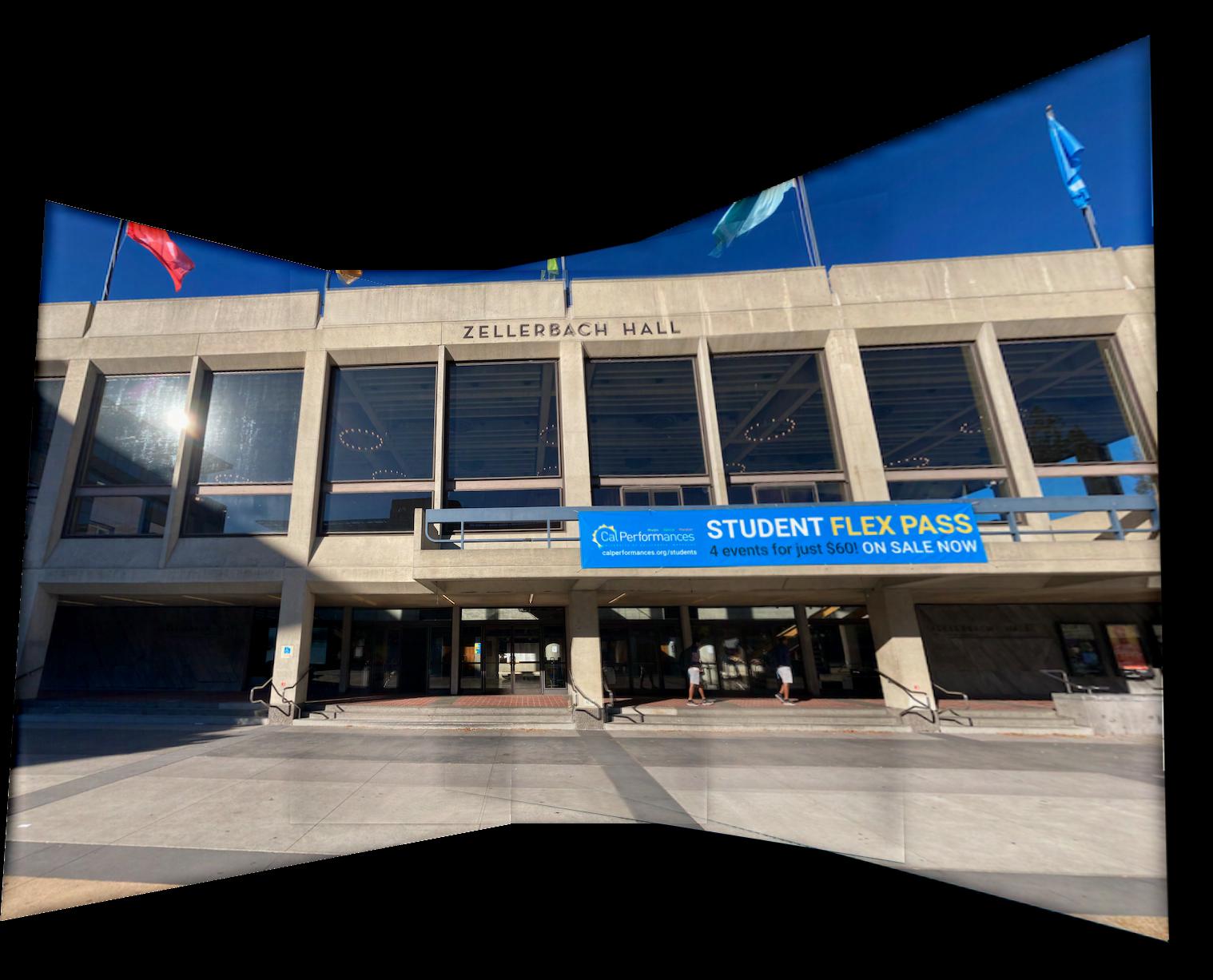
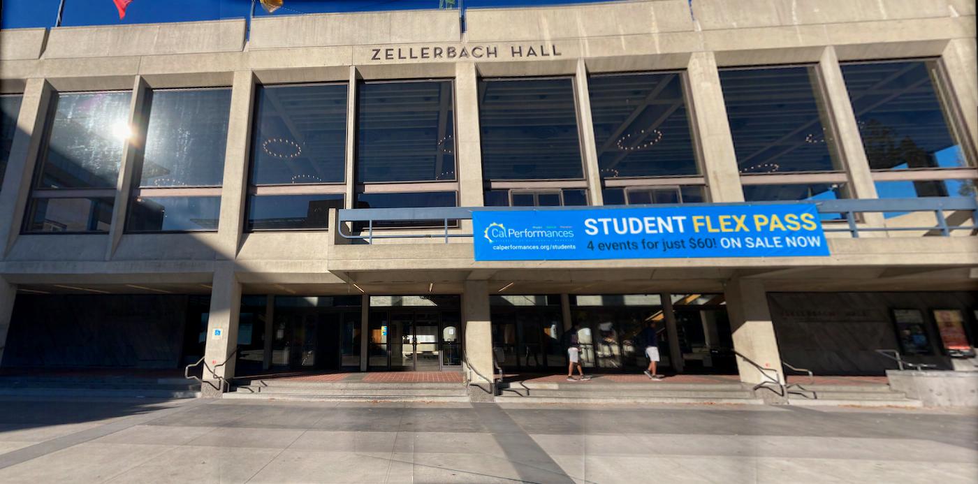
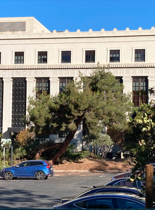
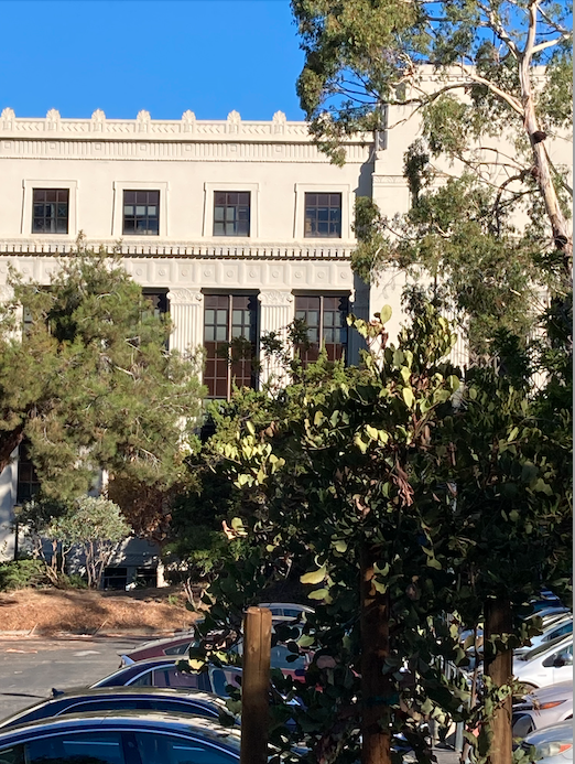
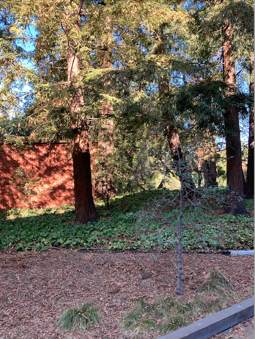
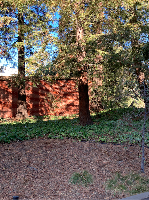
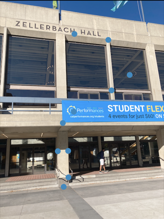
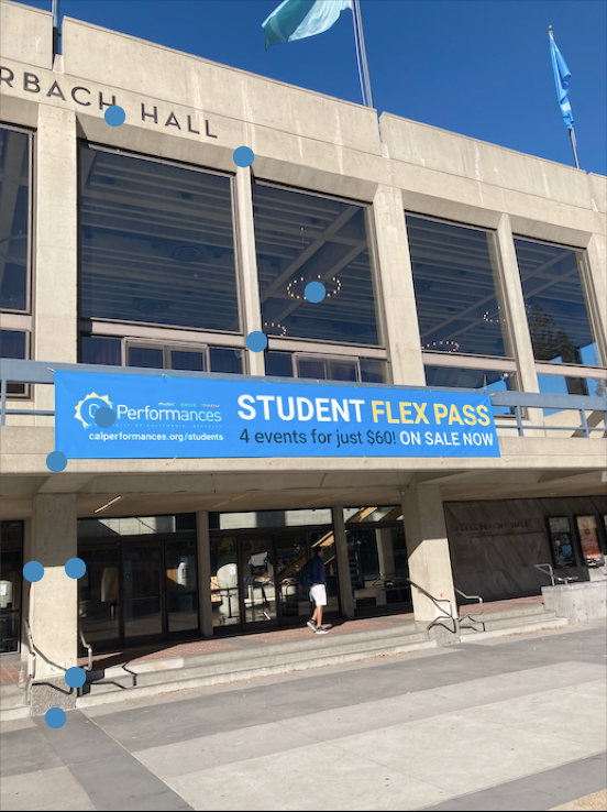
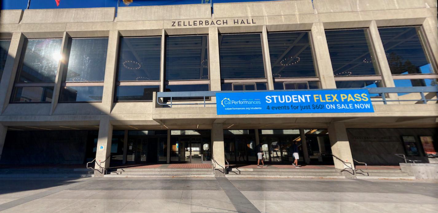
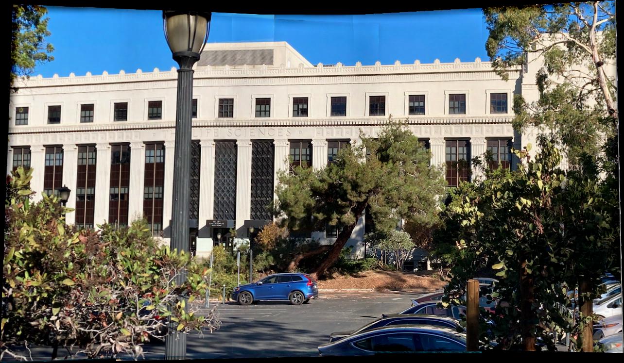
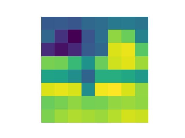
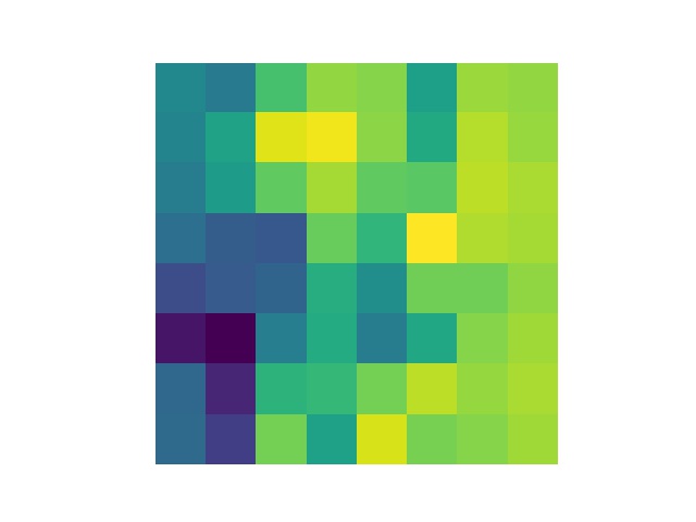
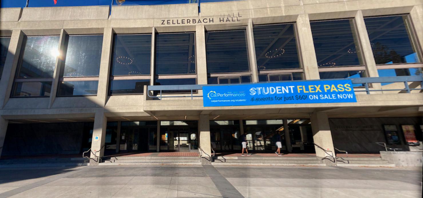
For this part we'll use a running example of two images from the Zellerbach collection. For detection and extraction of course we process the two images independently, it's only in the matching phase that we compare the two. Consider the below two images:
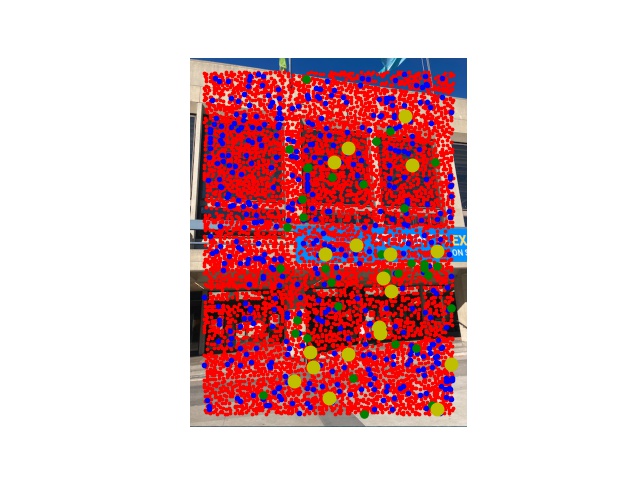
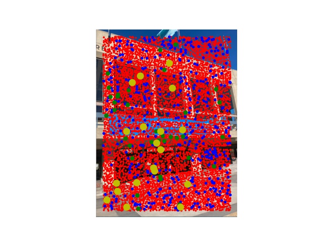
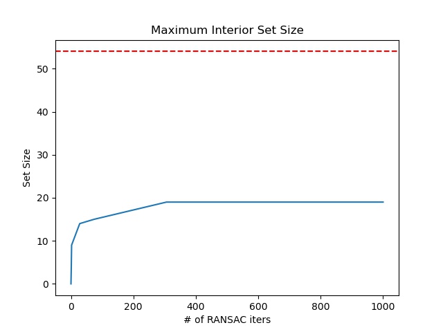
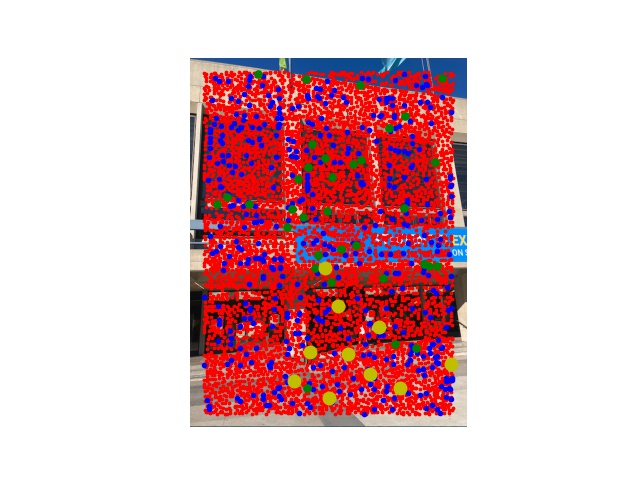
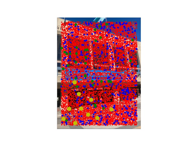
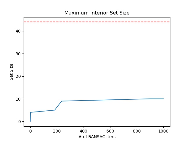
The red dots represent the corners as identified by the Harris Corner Detector (min_distance=1, edge_discard=25). ~8000 of these are detected for our 521 x 694 image. The blue dots are the top 500 resulting from the adaptive non maximum supression algorithm (largest non-dominated radius). The ~50 green dots are the points with a matched neighbor in the other image (1 - nn_1_diff/nn_2_diff > thresh=0.5; Feature visualizations in Part 3). We go through the matching process iteratively in the order of largest non-dominated radius in the first image and delete candidates from the second image as they're claimed as partners. The ~20 yellow dots are the inlier points found by RANSAC and ultimately used to compute the homography (Standard 8 degree of freedom least squares). The graph next to the images above describes the size of the best inlier set (tolerance 1.5px) that RANSAC found over iterations (Randomly try subsets of 4 points, compute homography using math above, keep the one which maximizes how many green dots map within tolerance to their correspondences).
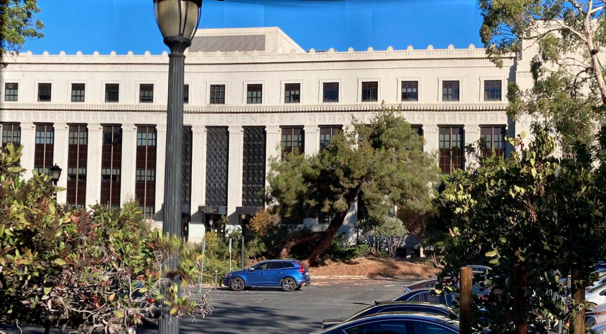
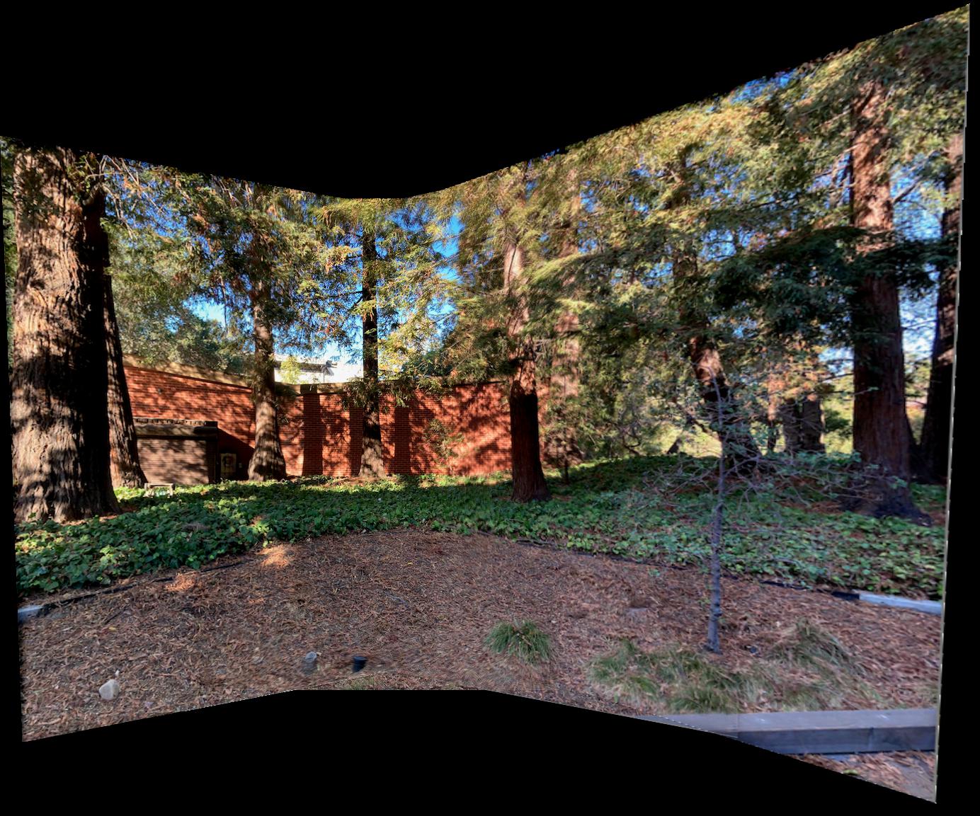
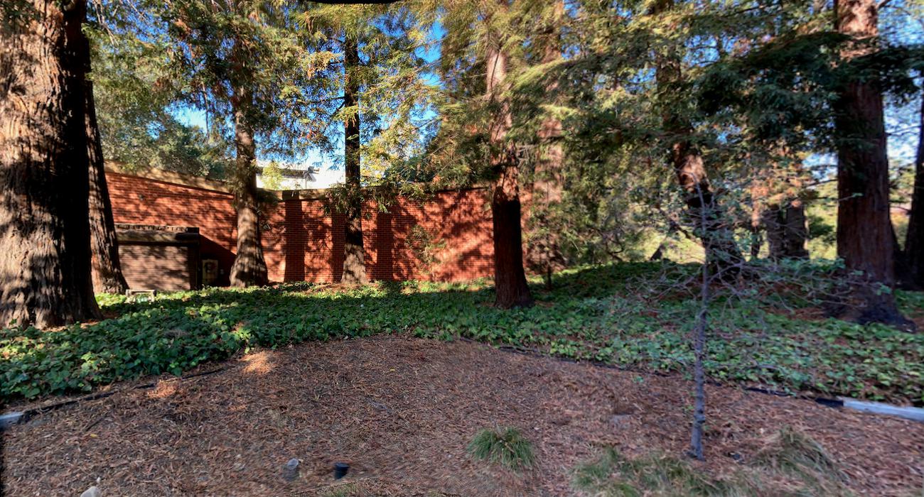
Below we show mosaics for the same three scenarios from before. For each scenario we first show the untrimmed versions then the trimmed versions. Left are copies of the previous manual correspondence results; Right uses auto matching.
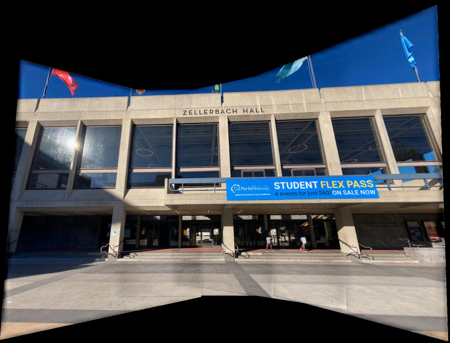

What I find really impressive is that the auto matching actually does better than the manual correspondences. I think part of this is that I provided only 6 manual correspondences per pair, here we end up with about 20 per pair. Furthermore, I definitely would have clicked a pixel or two off meaning my correspondences are not much better quality than what RANSAC selects. For qualitative evidence of the above claim checkout the following zoom ins. Again left is manual right is auto match. Moral of the story seems to be with least squares a greater quantity of potentially a little more noisy data is superior.


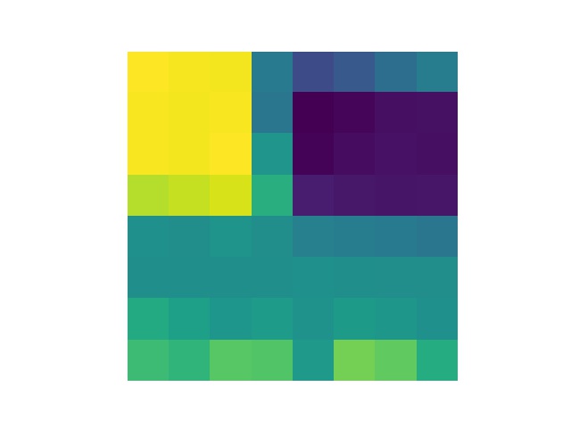
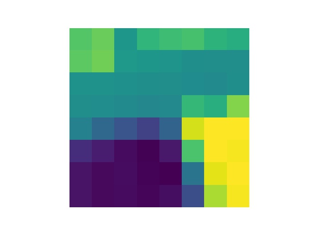
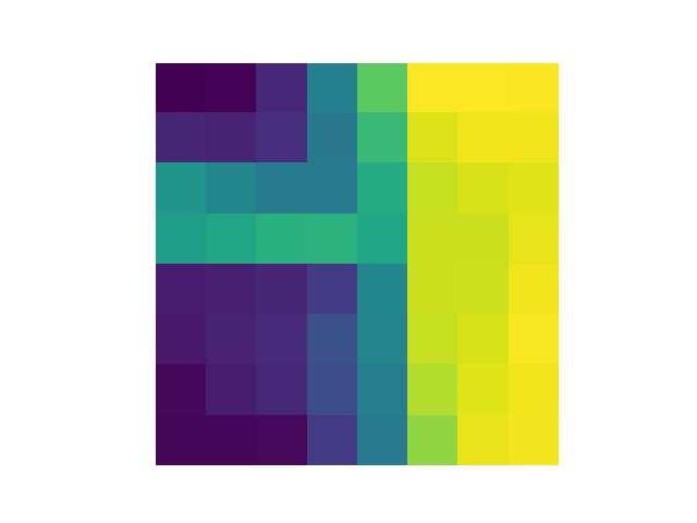
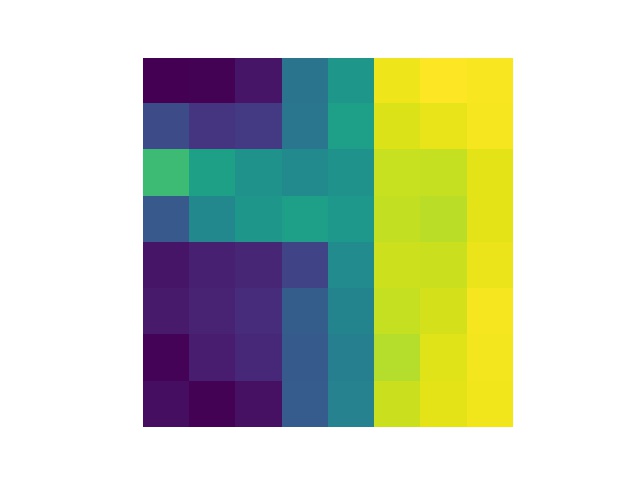
As a bell and whistle I implemented rotational invariance for features. The above examples were without this feature, now we'll evaluate the benefit of this features. First to develop intuition for what's going on consider the pictures below. In the rotated feature patch the gradient is always in the pure x direction. The feature distance metric I used was simple euclidean distance, which is obviously affected by rotating either image.
Below are the new locations we match and select via RANSAC. And below that a comparison of the mosaic generated for Zellerbach without rotational invariance (Left) and with (Right).
It actually performs a good bit worse mixing up most of the correspondences in the upper half of the image. I think the reason for this is actually quite explainable. I roughly maintain orientation between images. Meaning an upper right corner of concrete ought to match with an upper right corner of concrete. When we make the features rotationally invariant it's possible it matches a lower right corner of concrete because when rotated they appear the same. This makes the matching stage more confusing and thus RANSAC will through out these inconsistent pairings. I conclude that for our use case rotational invariance is not a good idea, but in panaoramas where we roll the camera it may be useful (unclear why you would do that though).
I think the coolest thing I learned from this project was how well auto matching based on these features could work. Overall we have a pretty complex multi step process for image stitching but the results in the end are fairly impressive given it's fully automated. Blending artifacts remain the most challenging (even if we blend a lighter and darker photo it still looks weird that the image randomly starts getting darker at some point). This last point is something I'm interested in learning more about how to resolve.