This project explored and put into practice the idea of recovering a homography transformation matrix, which is a three-by-three transformation matrix with eight degrees of freedom (the bottom right matrix value is set to one). The steps taken to recover the homography transformation matrix are explained in more detail under the “Recover Homographies” section. Using the computed homography transformation matrix, we can warp each respective image so that identified image features from the source will match the destination’s feature locations. After warping, the images are ready to be blended to produce a mosaic. Additionally, another application of recovering a homography transformation matrix and warping an image is image rectification which is used to take an identified planar surface in the image and warp the image to make the plane parallel with our perspective plane of the image which is called “frontal-parallel” in the project spec.
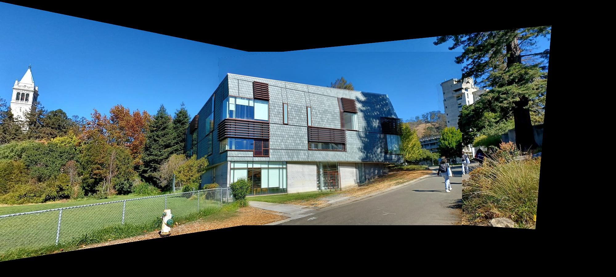
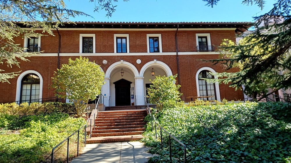
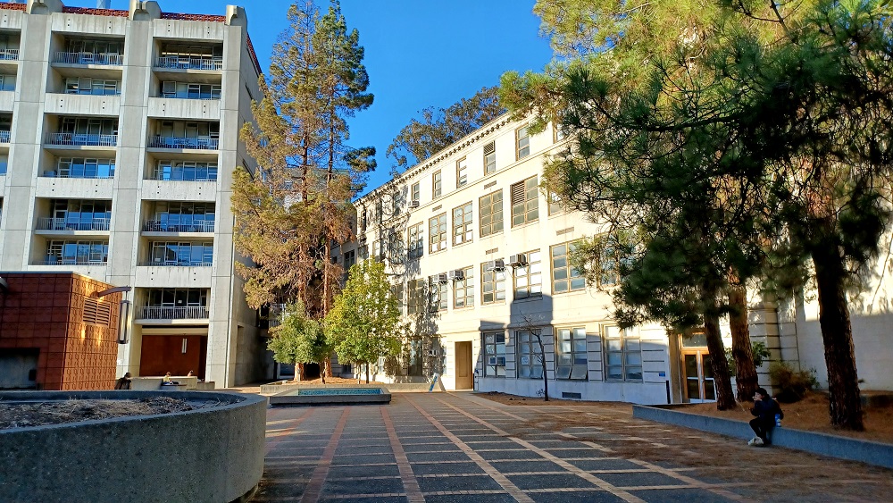
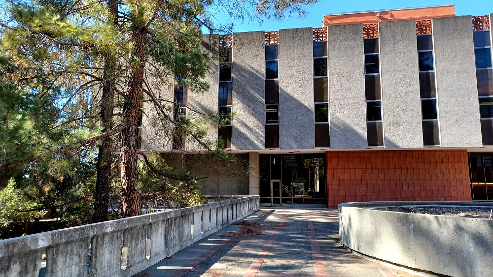
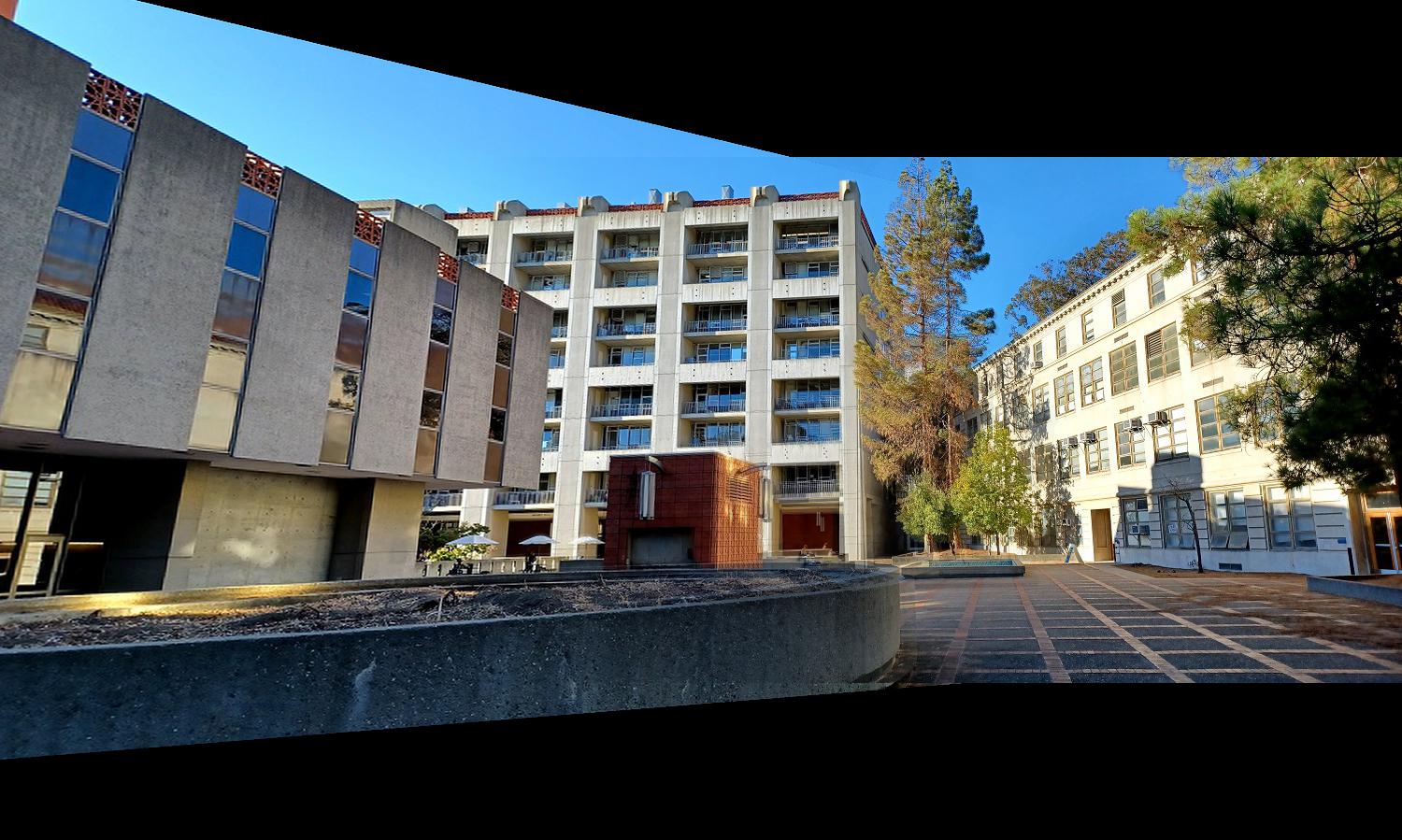
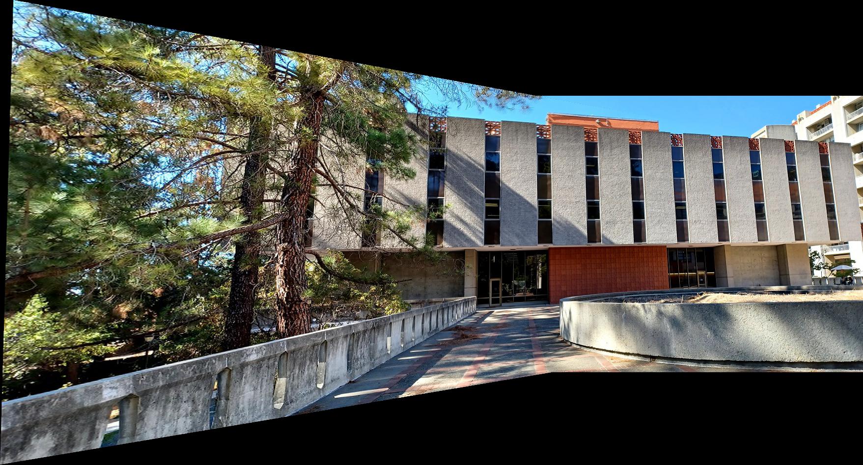
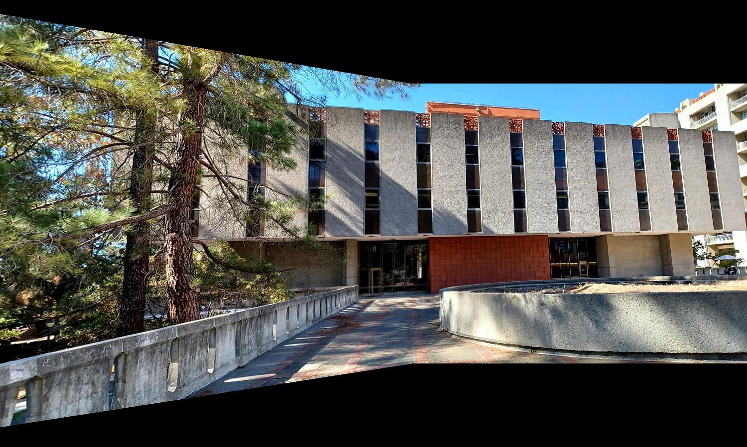
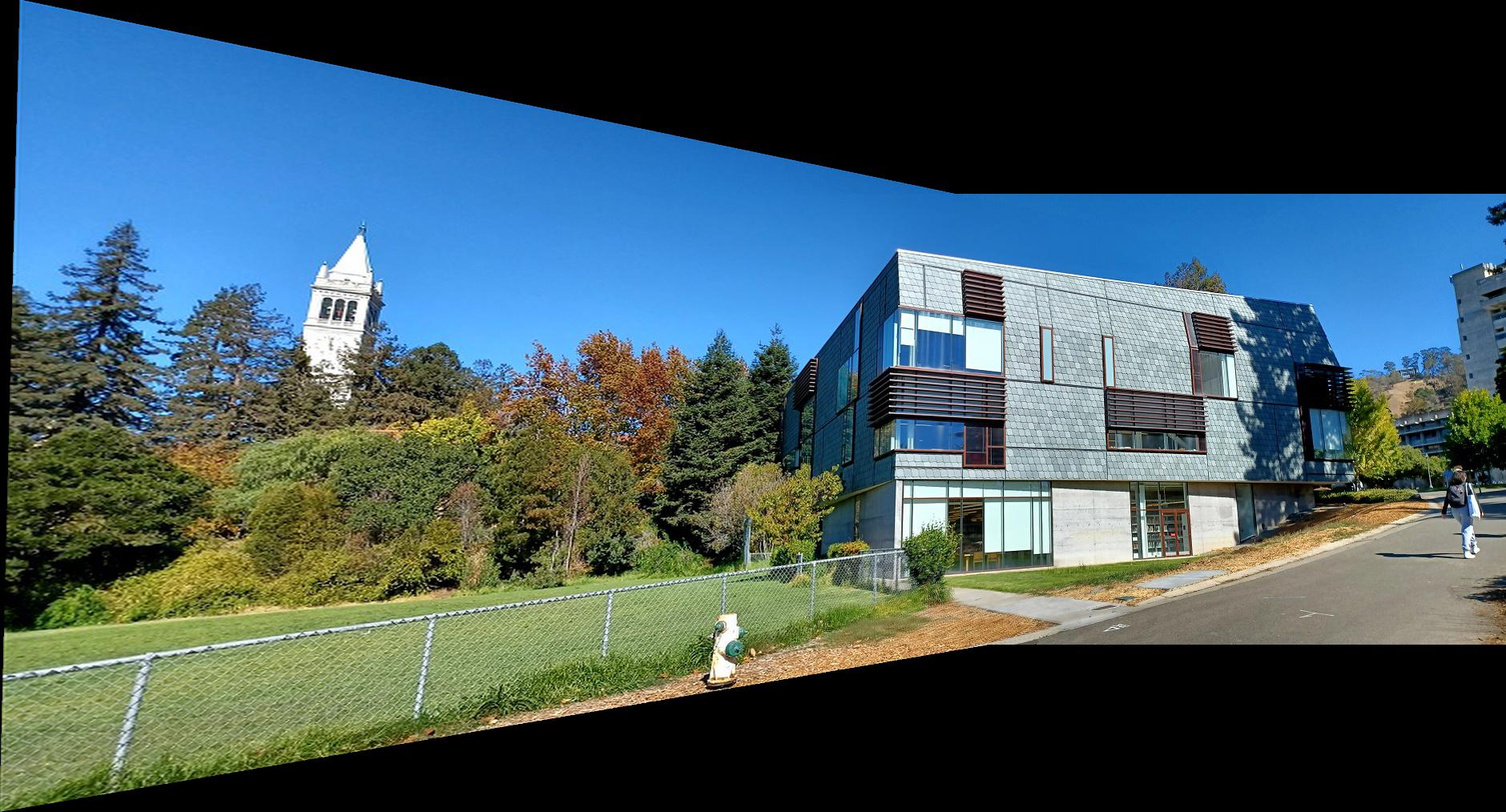
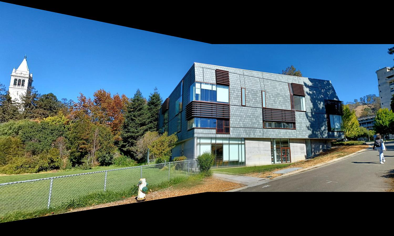
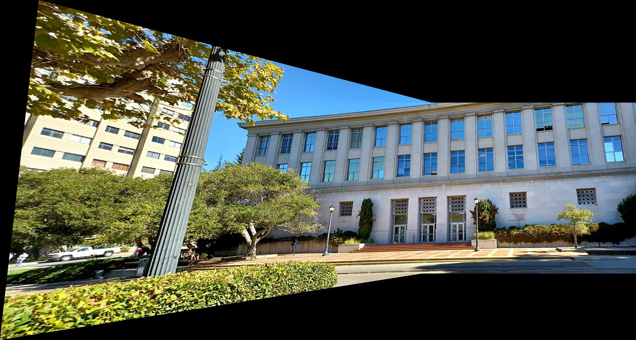
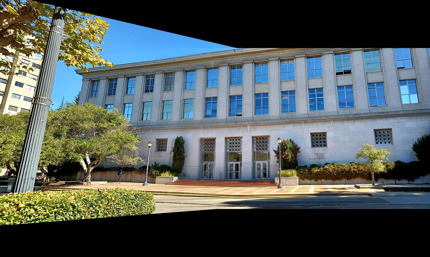
In order to produce the blended mosaics of images or rectify planes in images, we first have to take several digital pictures on which to perform the operations. Below are the digital images I took which will be used in each section. Their use case (i.e. image rectification or mosaics) is identified by the subheading under which they are displayed. Images used for producing each mosaic were taken from a single point of view (as best as possible) and the second image in each mosaic is used as the reference image from which the other two images are warped to match the identified features shared across all images. My code, however, is capable of supporting an arbitrary number of images (see “Recover Homographies” section for details) as long as a reference image is specified, which is used to warp all the other images to the reference feature coordinates.
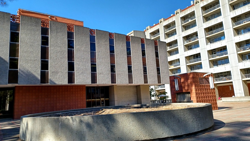
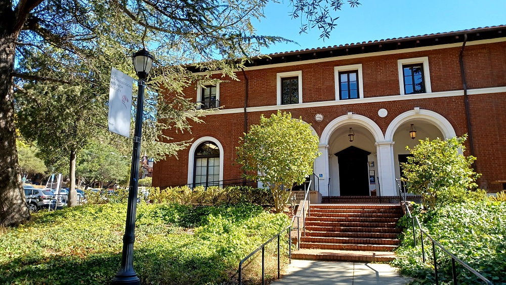
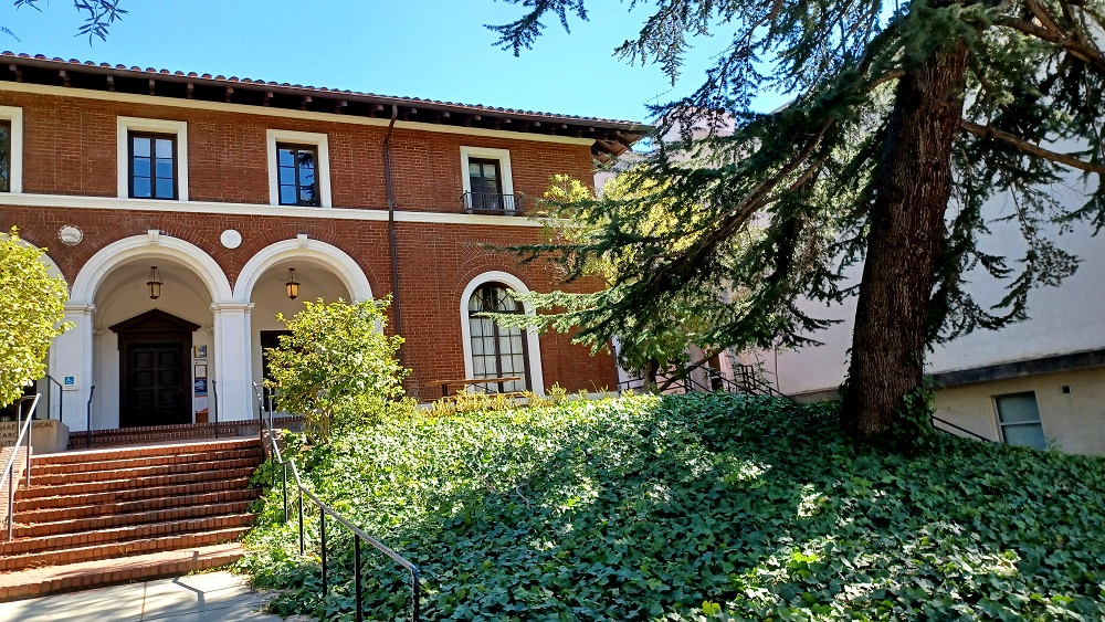
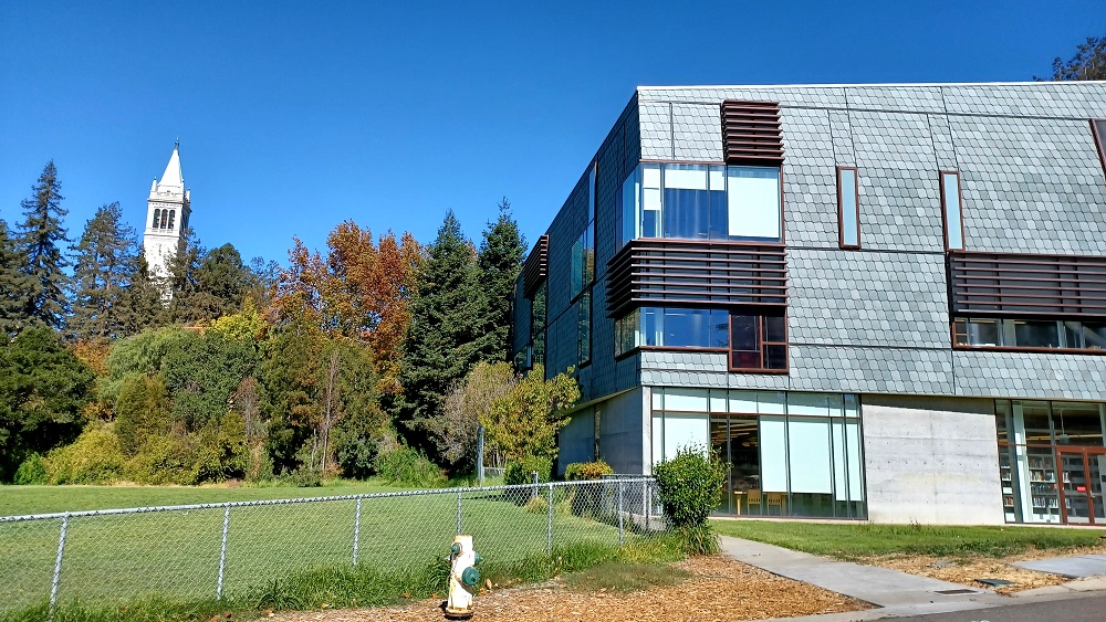
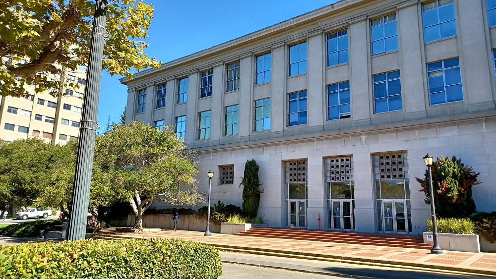
Images Used for Image Rectification


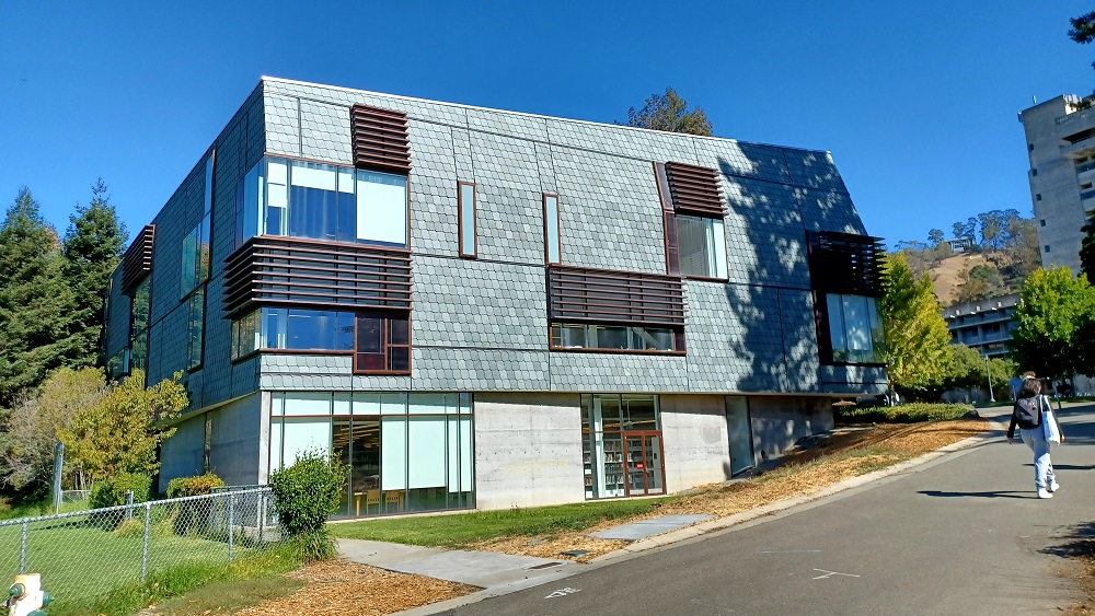
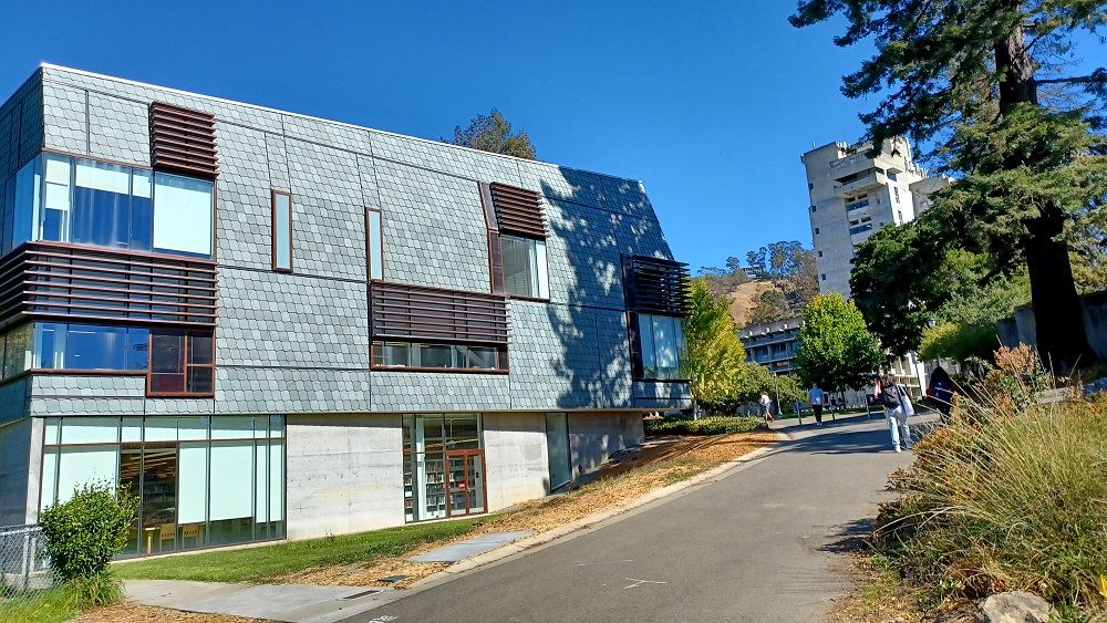
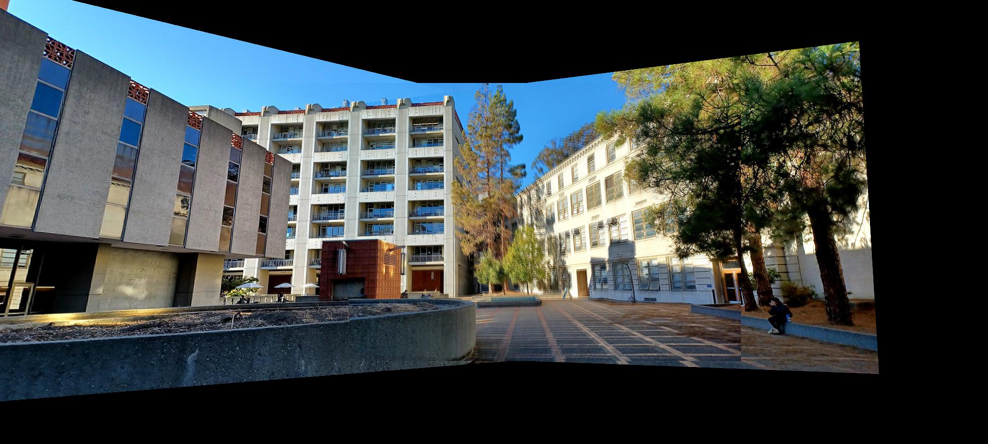
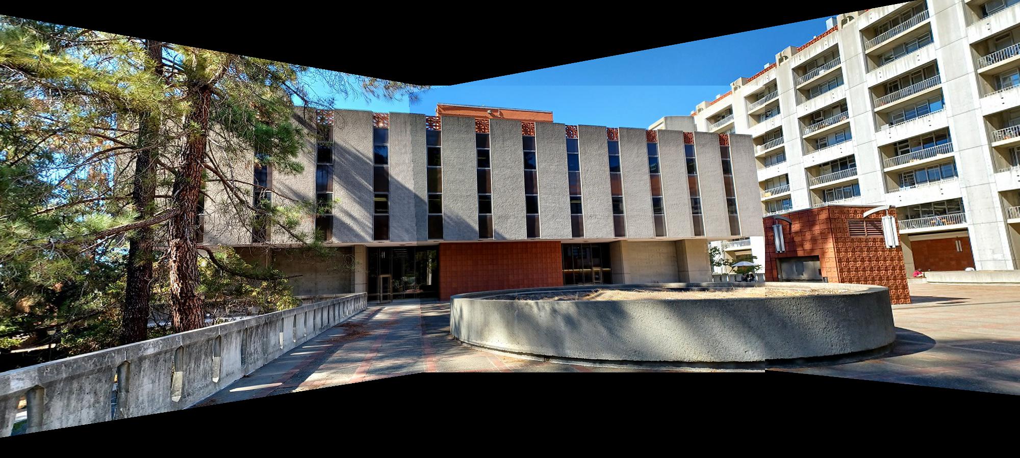
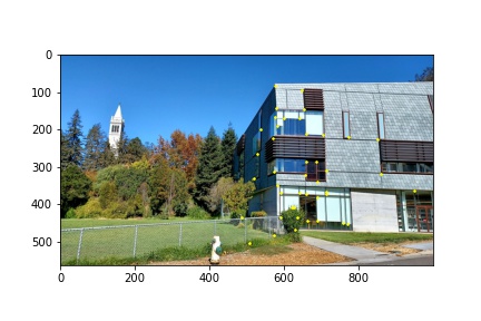
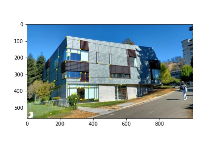
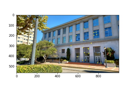
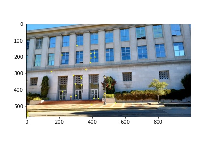
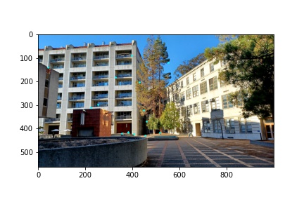
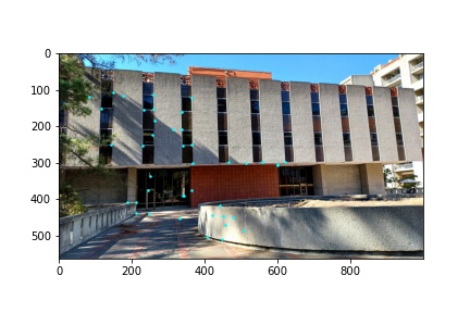
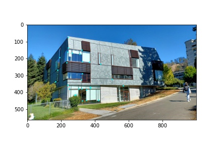
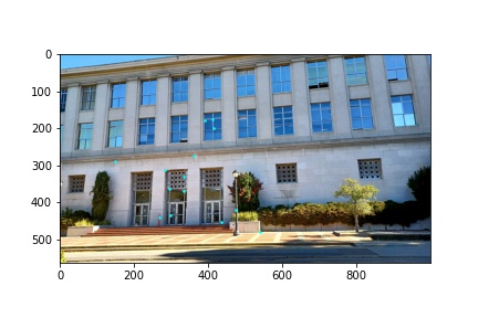
Images Used for Making Mosaics


In order to recover homographies, we need at least four correspondence points to be defined between two images, one being the source image and the other being the destination image into which the homography transformation matrix will warp the pixels from the source image (performed in the “Warp the Images” section). This is because our homography matrix has eight degrees of freedom, and each correspondence coordinate provides two values, an x and a y, so only four points are needed; however, additional points can improve the accuracy of the image warping by computing a better homography matrix since selecting the exact pixel values for the correspondence points between the two images is very difficult. By using more points, the homography is computed using least squares to minimize the error for the homography matrix. Thus, the more points used, the less likely the image warping and subsequent mosaic will be prone to significant errors. I have outlined the steps for computing the homography matrix below which assumes that the first step of manually defining at least four correspondence points on two images has been performed. I found this section to be challenging in rewriting the provided homography transformation equation offered in class into the form Ax=b with x containing the unknowns for our homography matrix.
We begin with the provided transformation equation offered in lecture. The coordinate vector on the right of the equation (p) refers to the source image correspondence points which are being transformed by the homography matrix (H) to produce the destination image’s correspondence points (p’).

We can expand this notation to view the values of the vectors and homography matrix in order to perform further computation. Here, x and y refer to the source correspondence coordinate and x’ and y’ refer to the destination correspondence coordinate. We note that x’ and y’ are scaled by w which cannot be assumed to be 1; thus, in the subsequent computation we will have to account for the w scaling term to extract the true destination points when performing image warping using the computed homography matrix.

From here we expand out the terms by performing matrix vector multiplication and extract three equations.


We observe that the first two equations share the w term which we can substitute into the first two equations as follows:


Expanding out the terms, we get the following:


From our previous assumption, since our homography matrix only has eight degrees of freedom, the i term in the homography matrix can be set to 1. This simplifies our equation by substituting 1 for the value of i:


Isolating the x’ and y’ terms now on the left side of the equation, we get the following two equations:


We can now rewrite these equations in matrix vector notation that conforms to the Ax=b format we desire. The resulting matrix and vectors are as follows:

The subscripts used in the above expression represent the correspondence coordinate to be used. Since we need a minimum of 4 points, then in the above notation, the values for the first point (x1, y1) should be appropriately substituted as well as for the second point (x2, y3), the third point (x3, y3), and the fourth point (x4, y4). However, we want to be able to process more than four points and compute least squares when determining the values of our homography matrix which are contained in the x vector. Thus, the above expression is generalized to accept n defined points, as denoted with the subscript n following the ellipses in both the A matrix and b vector. We solve for the unknown homography variables as follows. I will use the abbreviated Ax=b notation for the following computations.
We start with the above defined matrix vector expression:

Where A is the n by 8 matrix shown above, x is the vector which holds the unknowns for our homography matrix for which we are solving and b is a n by 1 vector that holds the destination x’ and y’ coordinates that are associated with each linear equation. We first multiply both sides of the equation with the transpose of the A matrix to produce a square matrix that is invertible (this is important for the next step)

We then multiply both sides by the inverse of the resulting matrix from the product of A with its transpose. The matrix is invertible since we multiplied A with its transpose. This will leave the identity matrix on the left side of the equation, isolating the x vector of unknowns and allow us to compute what the values of those unknown variables are given n correspondence points.

From here, we simply place the corresponding values in the found x vector into the appropriate locations for our homography matrix and return H (our homography transformation matrix). This is the procedure I implemented in my computeH function which returns the homography transformation from the correspondence points in image1 (the source) to image2 (the destination).
Now that we have computed the homography transformation matrices for each image, or only a single image as is the case for image rectification, we can warp the images given the homograph transformation matrix. In its current format, the homography transformation matrix will translate coordinate values from our source image, the input image, to some new warped coordinates which I will call the destination image. This would result in forward warping the image; however, in order to avoid aliasing on the warped image, my warp function first finds the inverse of the homography transformation matrix so that I can inverse warp the image and use interpolation to sample the original image for each warped pixel’s coordinates.
More specifically, my warp function first begins by initializing three new canvases, for the red, green, and blue color channels of the warped image, that are of the same dimensions as the input image. Then for the three color channels of the input image, I define interpolation functions each using RectBivariateSpline. I then get all of the pixel coordinates in the image in order to warp each of those pixel coordinates and perform the subsequence sampling of the original image. Before doing so, I find the inverse of the homography transformation matrix such that the transformation matrix will now convert the pixel values on the warped image’s canvas to the appropriate pixel values to be sampled from the original source image (before inverting the transformation matrix, it would take the pixel coordinates of the original source image and convert them to the coordinates associated with the warped image). The result of inverting the homography transformation matrix to perform inverse warping is more clearly shown in the following equations.


Inverting and applying the homography transformation matrix on each pixel coordinate of the warped image canvas, I proceed to sample the original image using the defined interpolation functions given the transformed coordinates. The sampled pixel values are then recombined to form the warped color image which is returned by the function. Additionally, my warp function can also return the mask associated with the warped image, or a black box on the white canvas representing where the warped image lies on the mosaic frame. This is helpful when blending the images together to form the mosaic.
The warped images along with their alpha masks for each of the mosaic images I used are displayed below to demonstrate that the homography transformation matrix and the warping function are working as intended.
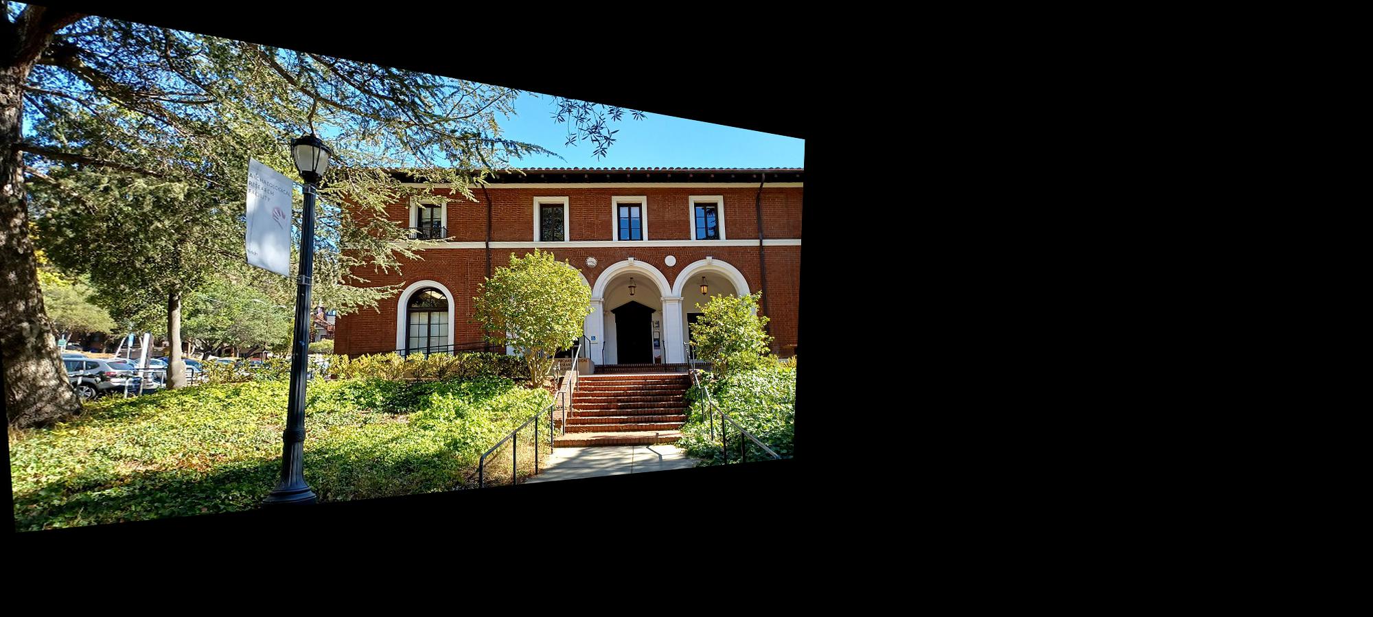
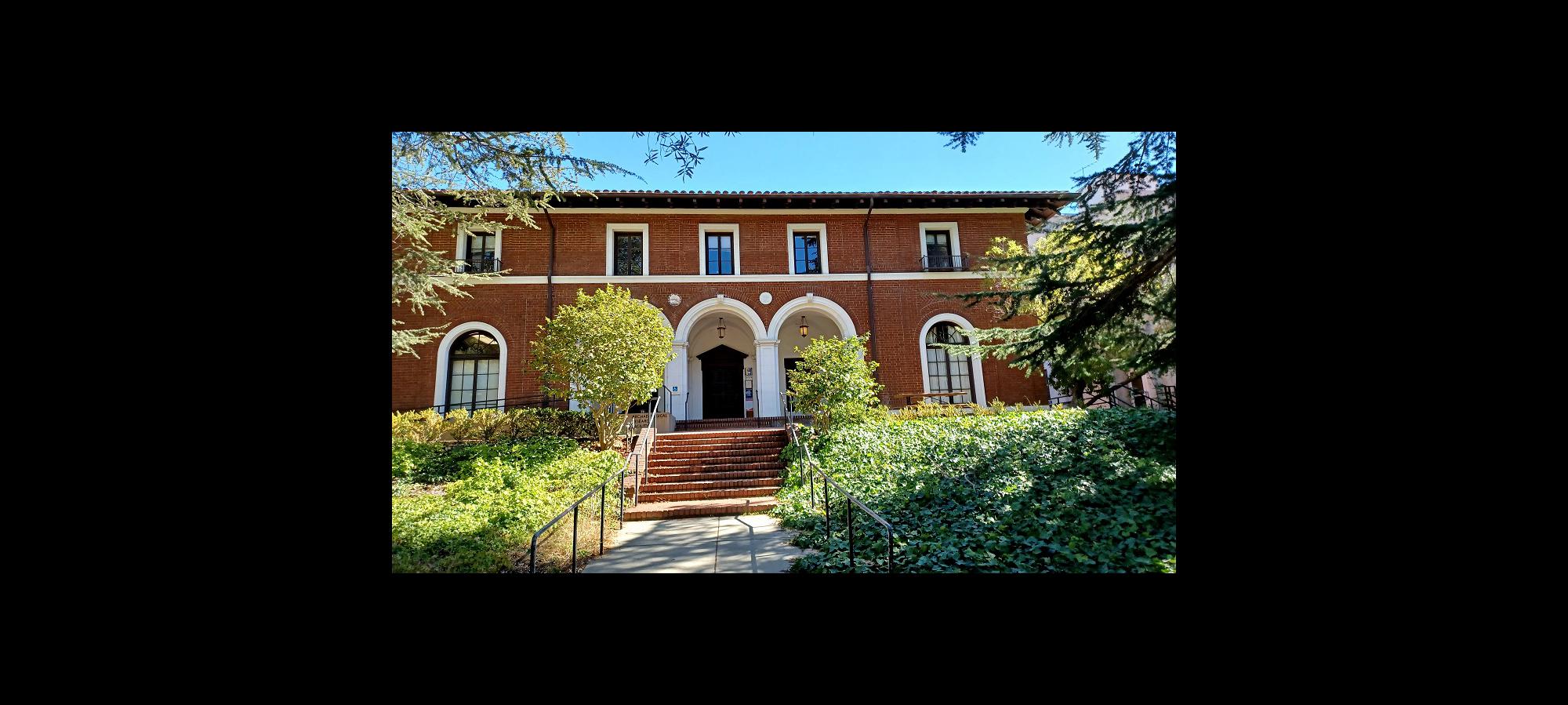
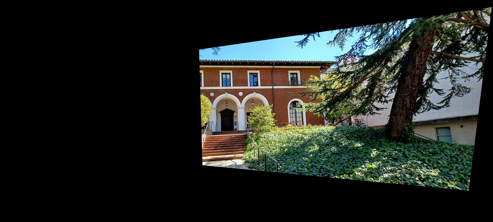

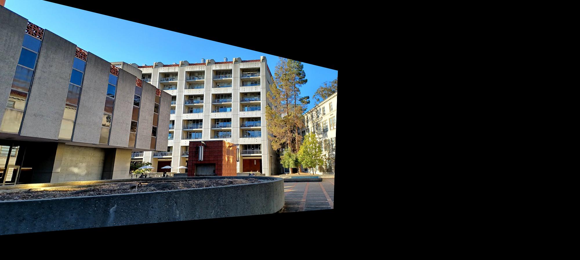
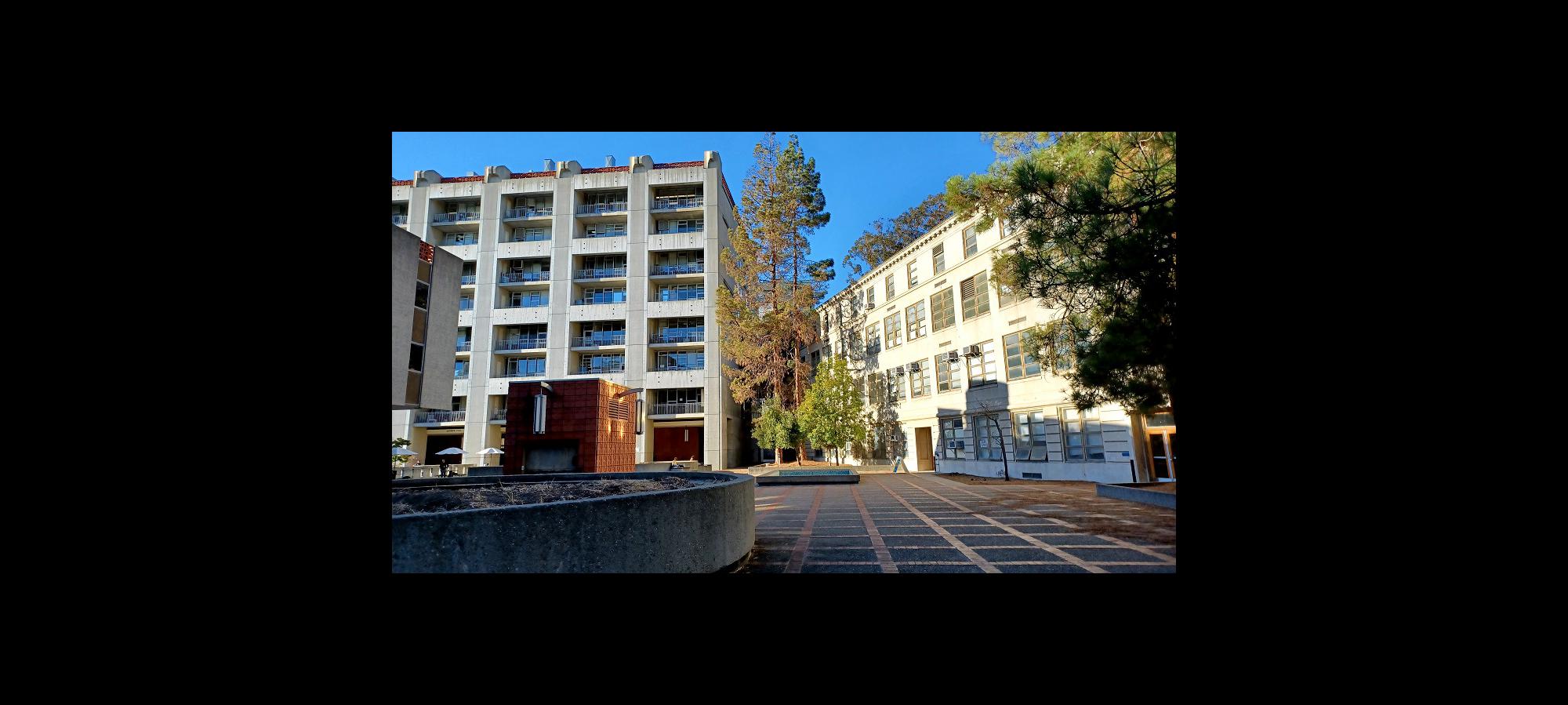
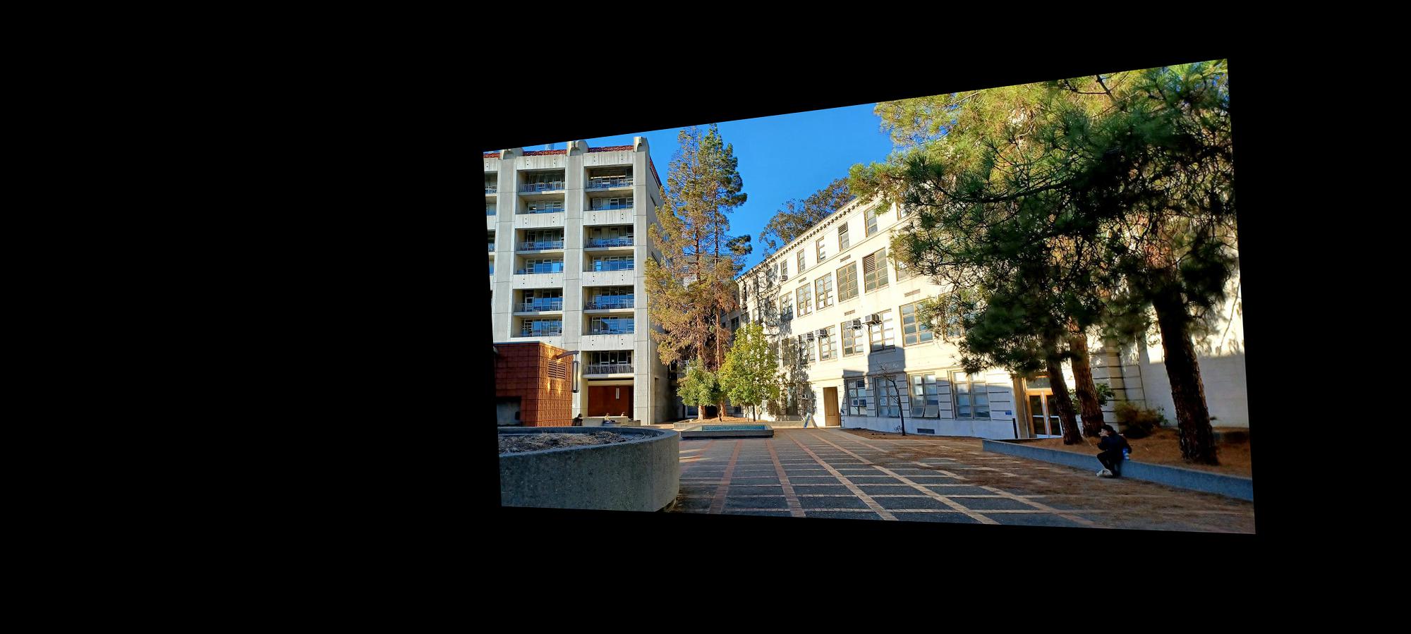

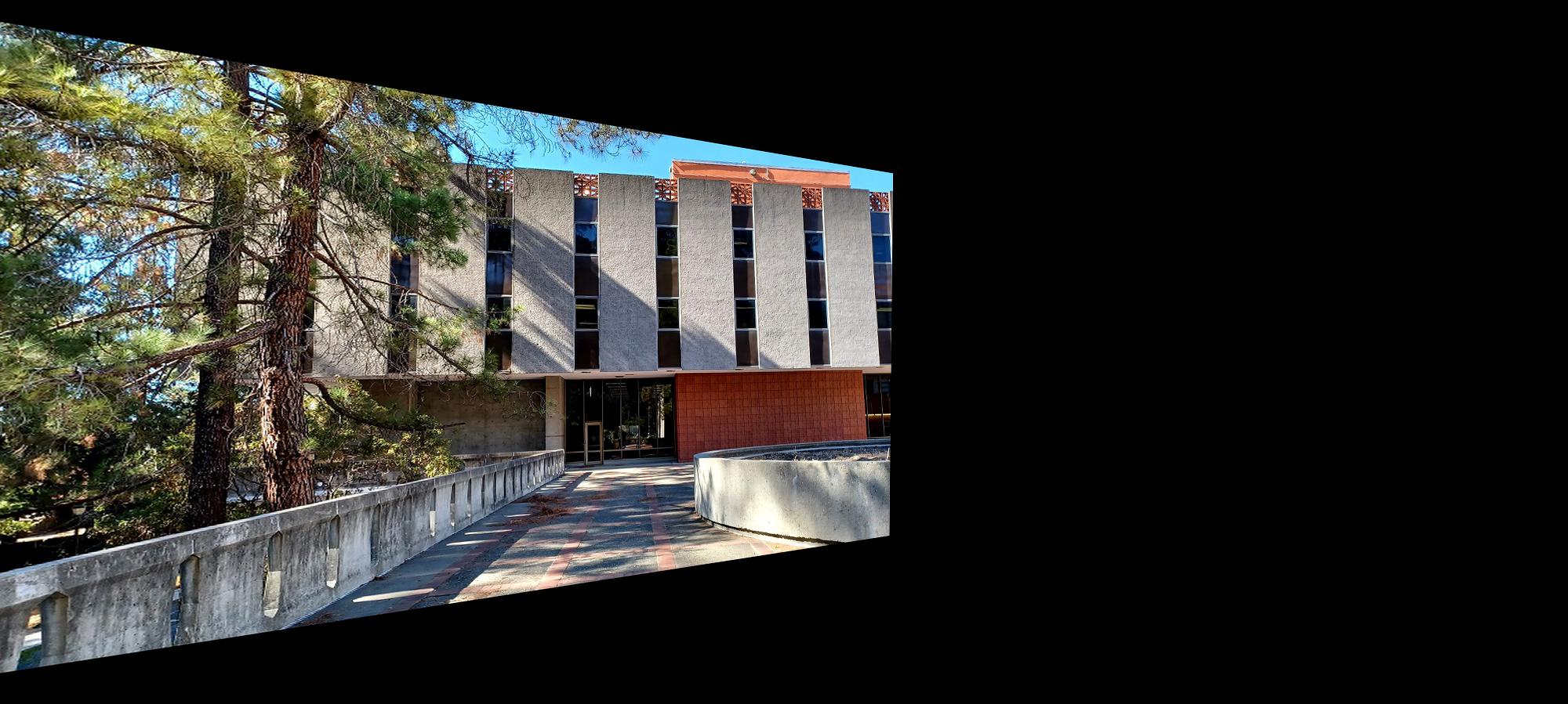
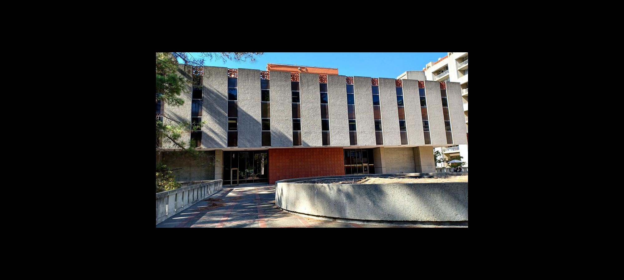
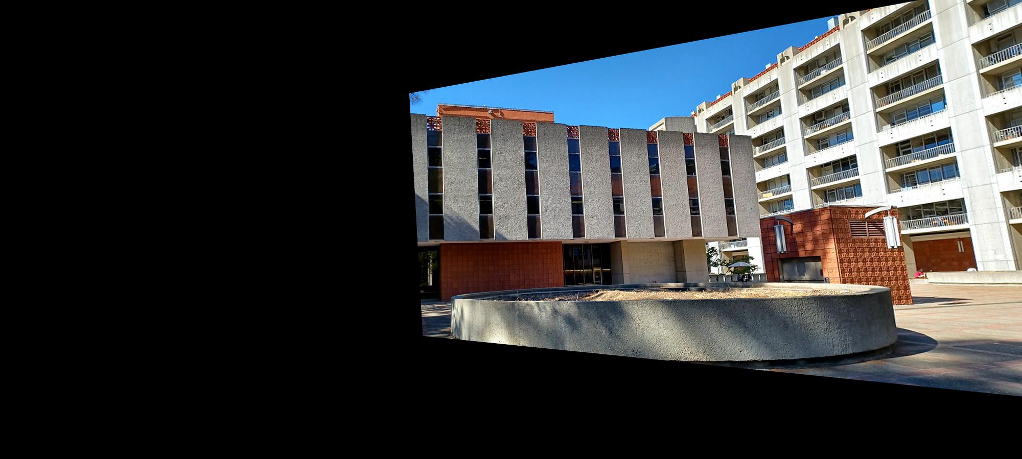

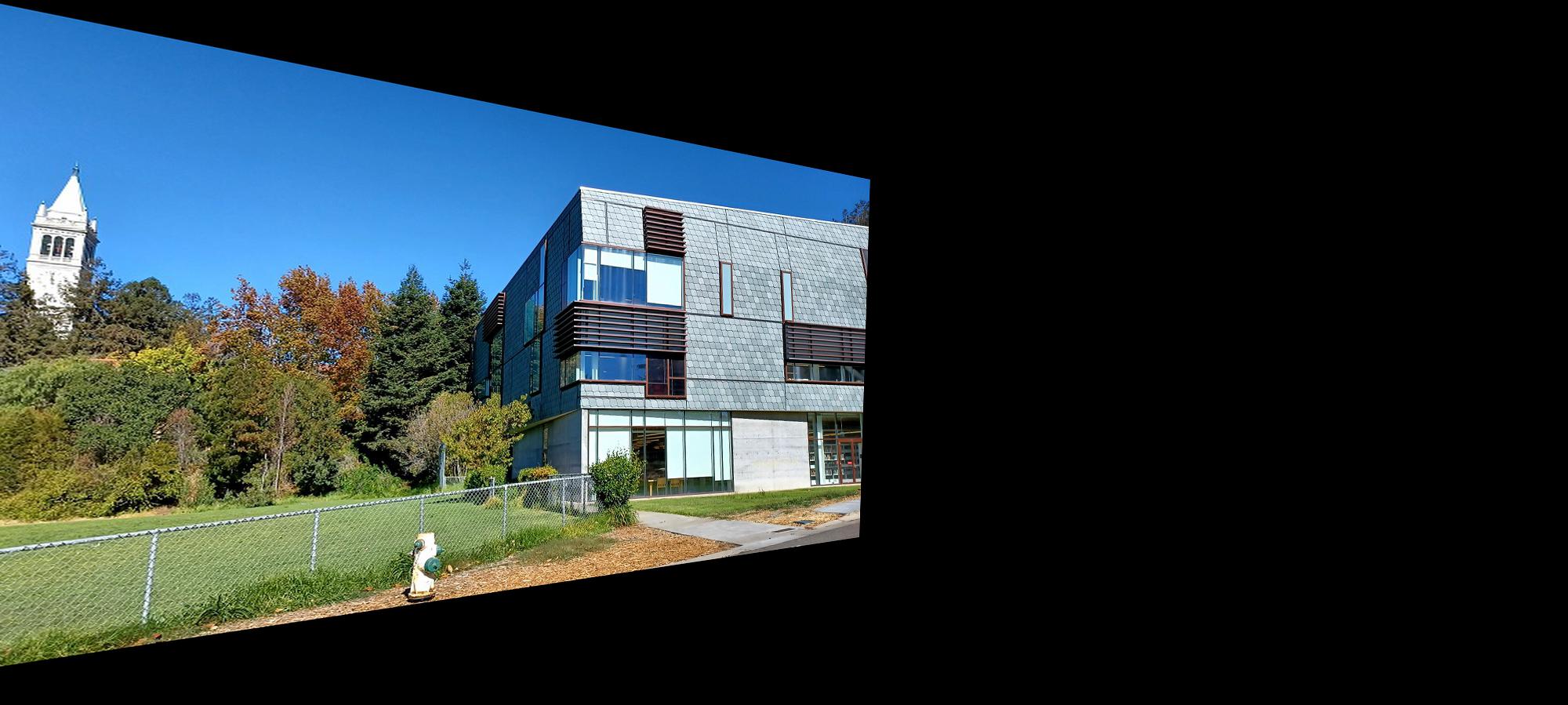
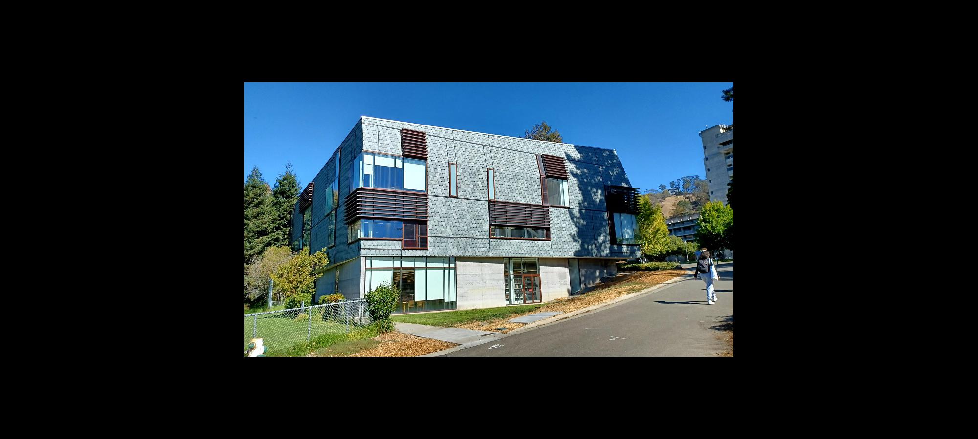
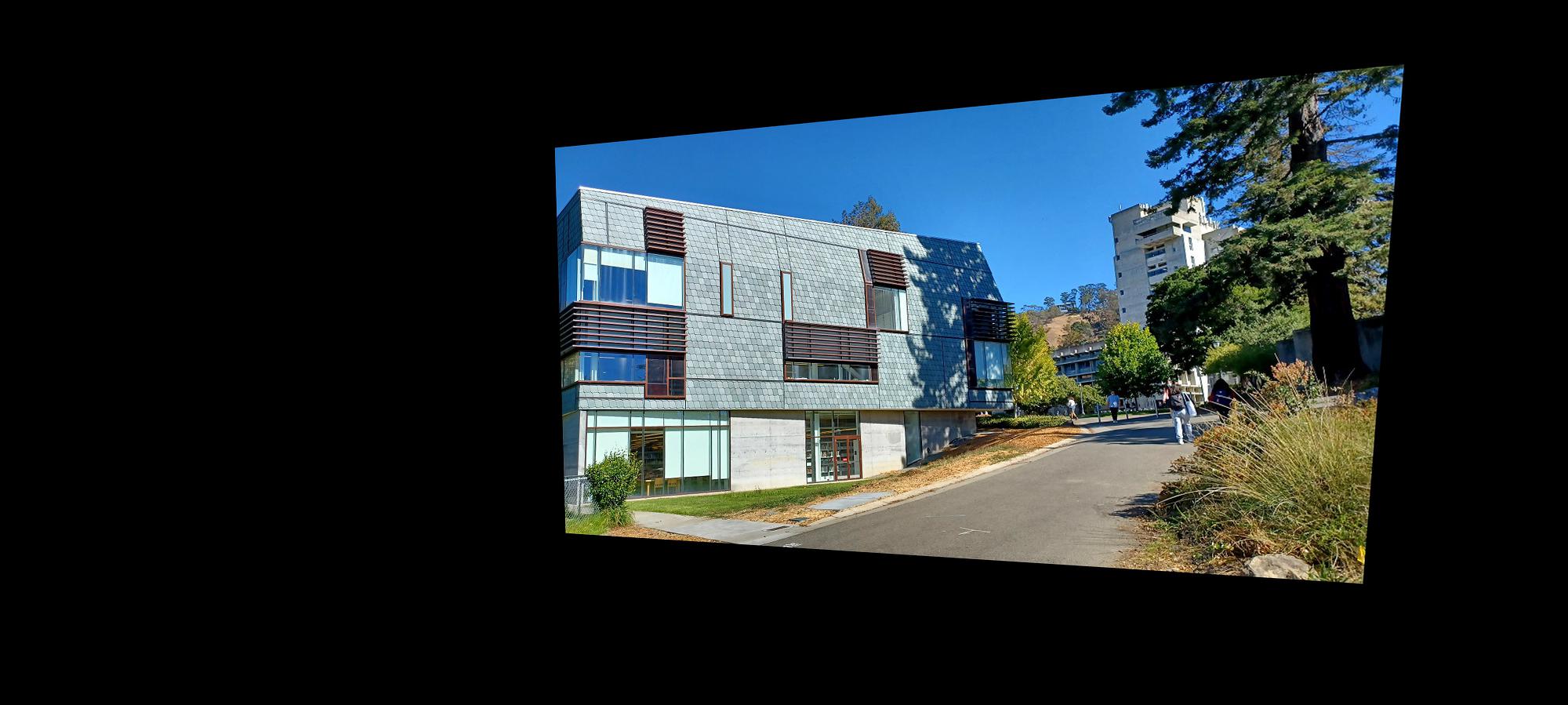

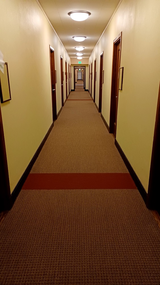
Image rectification uses the same functions we built for finding the homography transformation matrix and warping an image using that transformation matrix but instead of defining correspondence points between two images, we identity a plane in the input image which we want to transform such that the plane in the image is now parallel with the image plane. It helps to know the geometry of the identified plane since the coordinates used to compute the homography transformation matrix are determined manually based on the anticipated geometry of the selected plane. For example, one of my rectified images was that of a hallway which was a carpet with rectangular patches on the ground. I know the rough dimensions of the rectangular patch and can then define the rectangular coordinates with which to compute the homography. This results in a warped image with the carpet feature plane parallel to that of the image plane. It also creates the perspective that we are now looking down on the floor rather than down the hallway even though a separate picture was never taken. Below are a couple of the images that I rectified.
I first began with an input image which we saw in lecture. This was my sanity test-case to make sure that the homography and warping functions were working properly and they did successfully produce the output image from lecture.
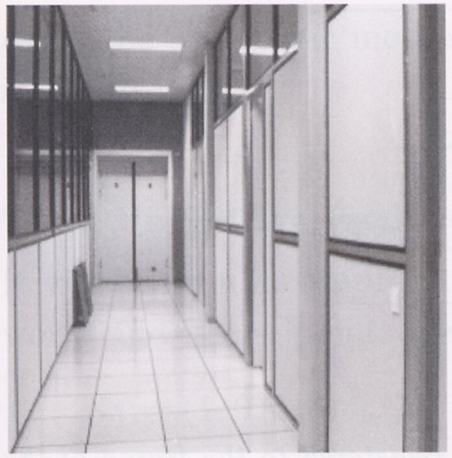
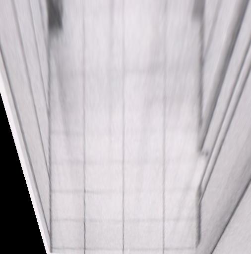
I then rectified the hallway image which I explained above, using the burgundy carpet patch as the rectangular plane on which I was going to rectify the image. The result seems very convincing as if the picture was taken facing down on the floor rather than looking down the hallway, although the black corners on the bottom of the image due to lack of information break the illusion. We can also observe that the pixels towards the top of the rectified image appear blurrier, in the original image, this was part of the hallway further away from the camera, so less detail was captured.
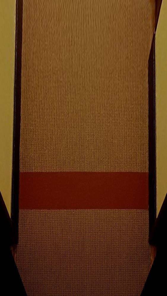
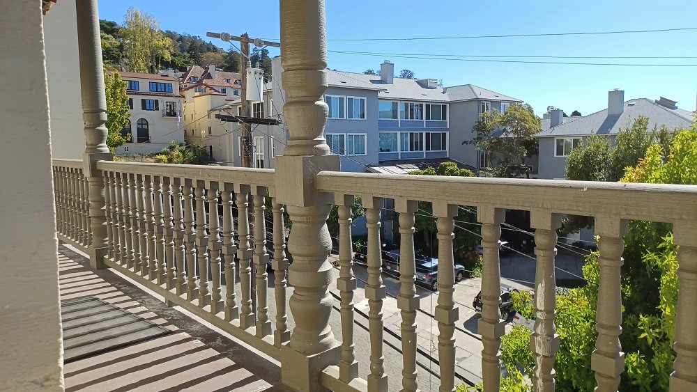
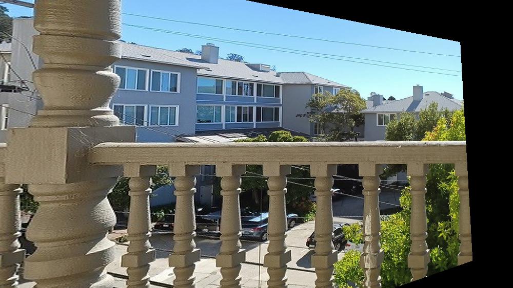
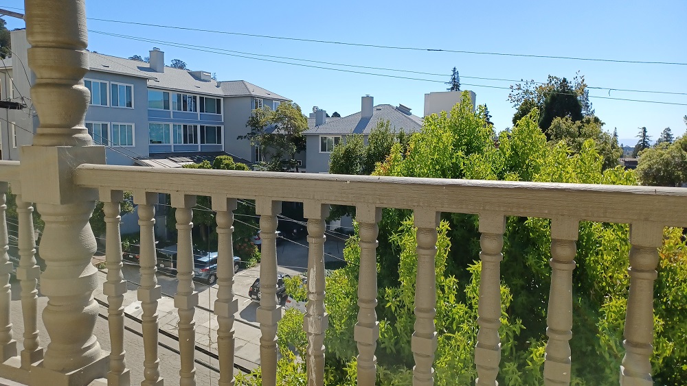
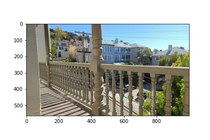
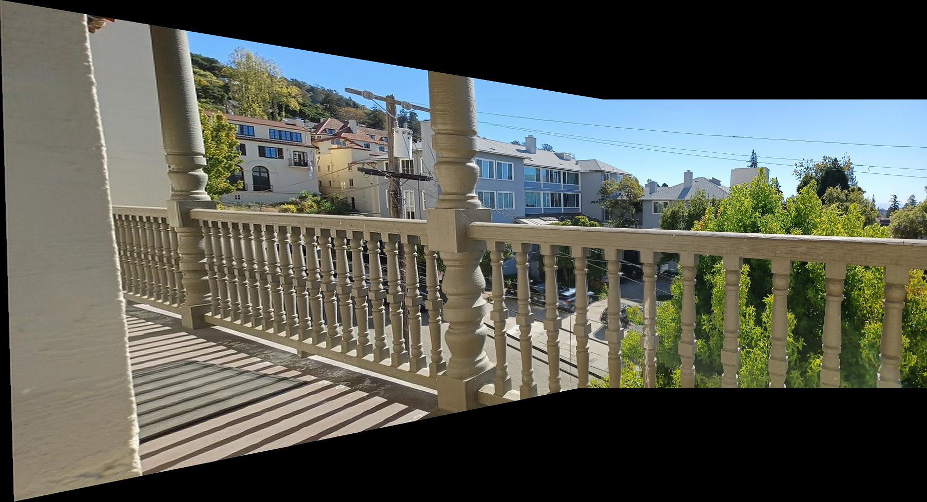
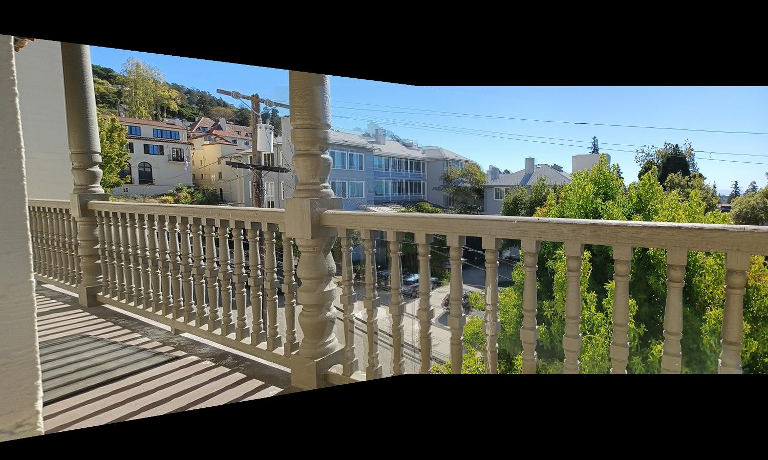
The second image I rectified was taken from a balcony on an angle. I decided to make the railing posts the plane on which to rectify. The results are viewable below.
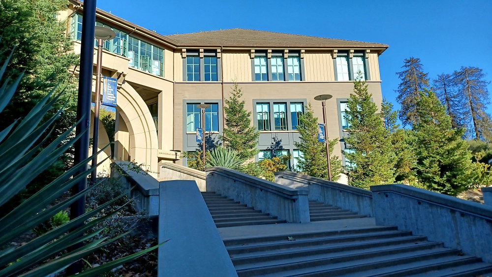
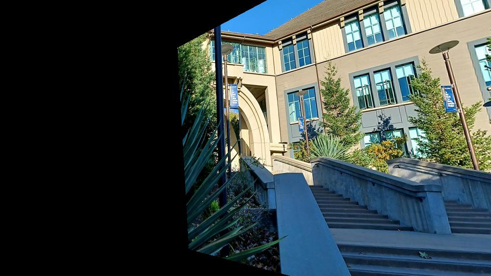
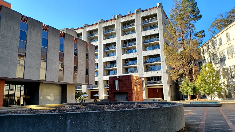
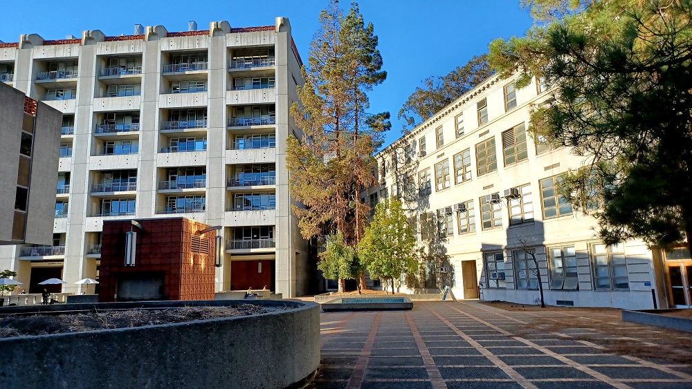
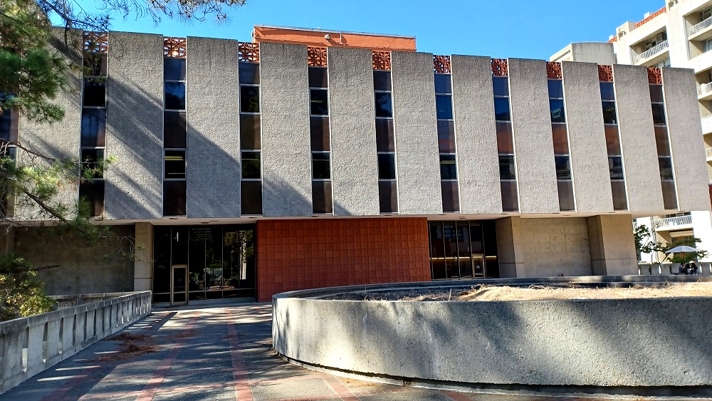
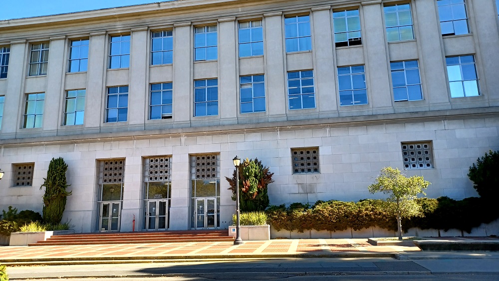
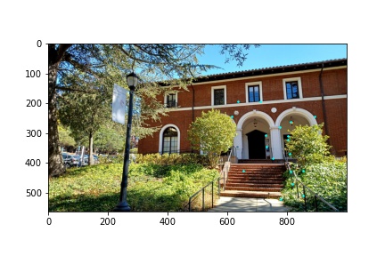
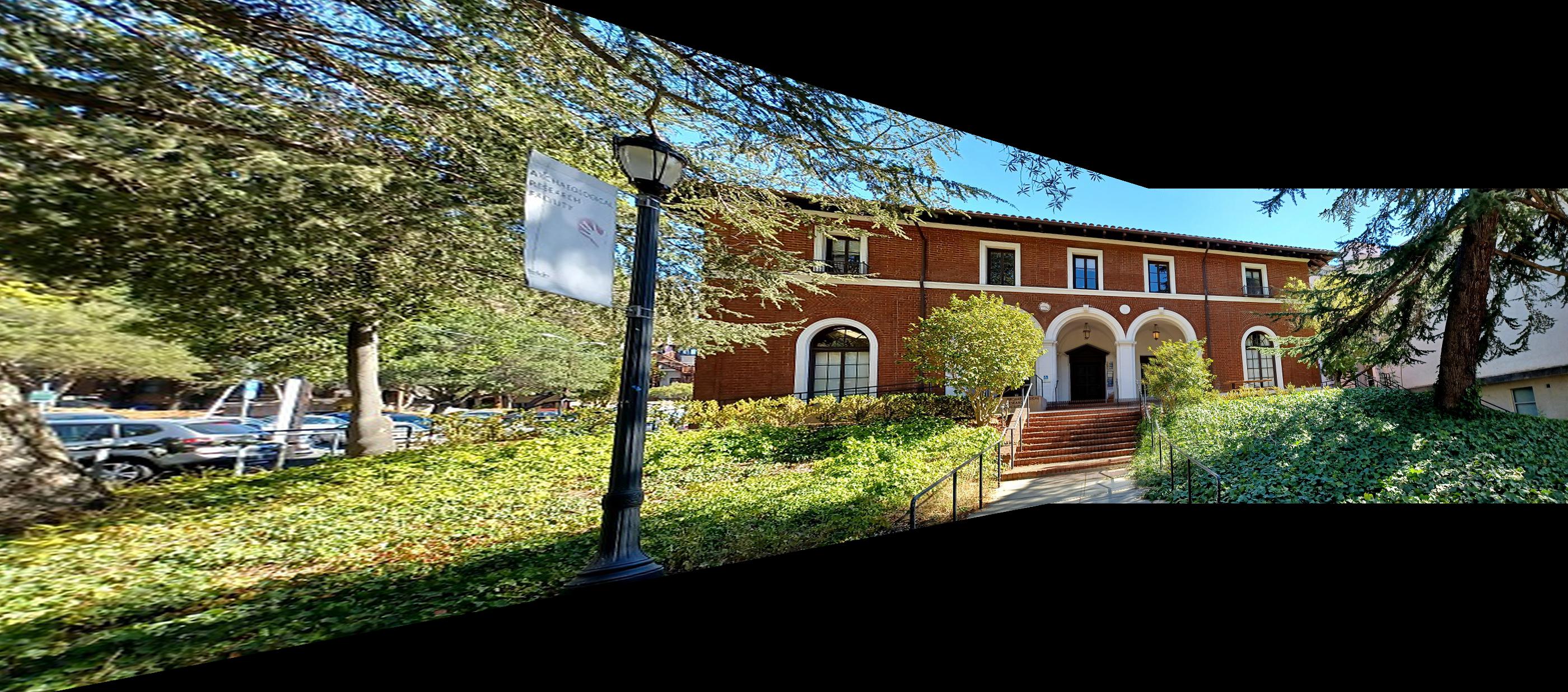
I also did a partial rectification of the bussiness school with the windows over the arch. The windows could have been more planar but then not much of the scene would be visible but we get a different perspective of the front of the building using rectification
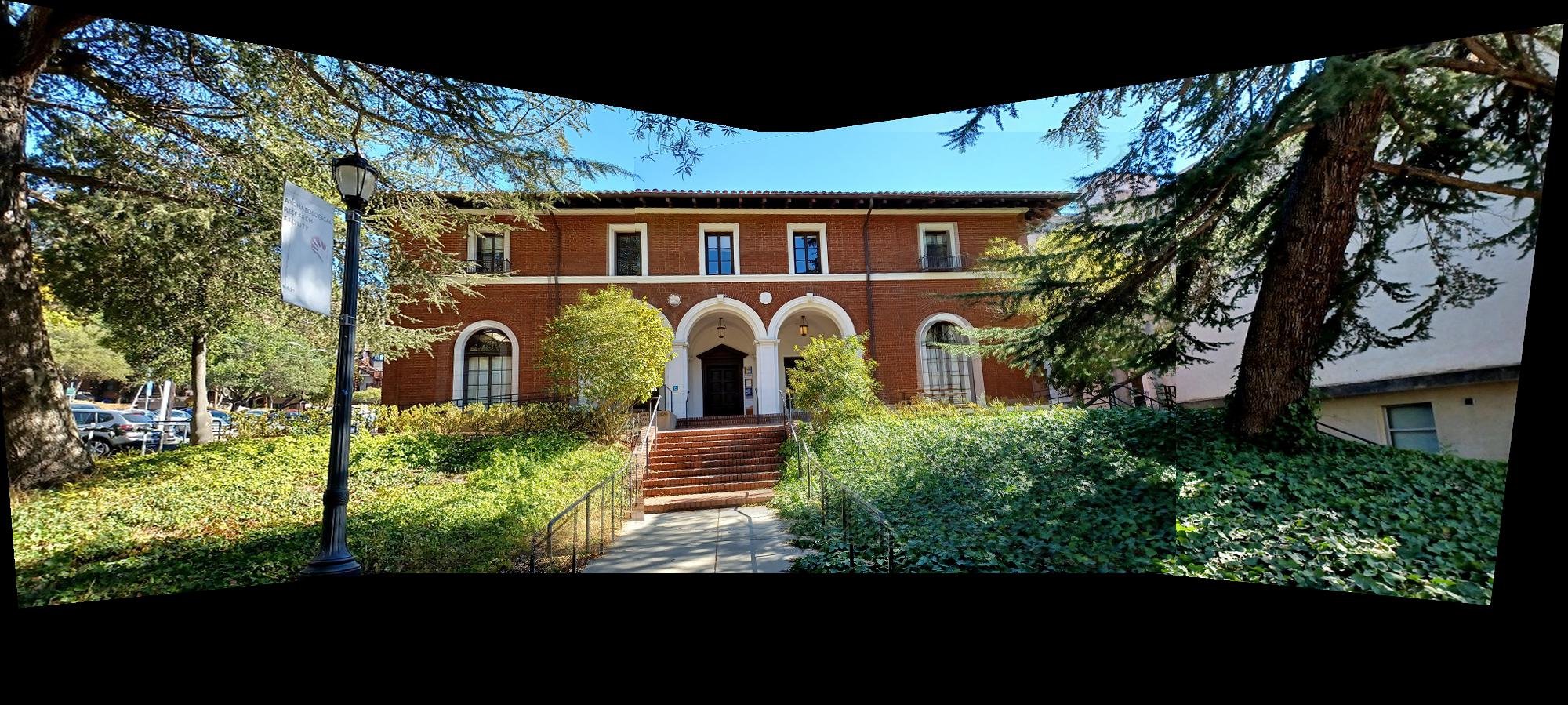
In this section, we take the warped images previously computed along with their warped alpha masks and combine the images to produce a mosaic. For my implementation, I applied a weighted averaging over the regions of the mosaic where the images overlapped as to make the transition between the two images less abrupt. I did this by first using the alpha masks for each of the images to determine where the overlap regions where and created a new alpha mask for that overlap region. I then applied a gradient weight on the newly created alpha mask so that the weights of one image would increase from 0 to 1 moving across the overlap region and the inverse was true for the other image in that overlap region. Though the weighted averaging using the alpha masks for each image did improve the overall quality of the mosaic, some of the blended frames are still somewhat visible due to two reasons. The first is the change in brightness of some elements in the scene. Unfortunately, I only have my smartphone as a digital camera and even on its manual picture taking setting, not all of the controls were really manual so image processing was still applied to each digitized image. This resulted in images with different brightness as well as other subtle filters applied to them (some kind of AI image enhancing feature my phone does while saving each image). The second is that not all of my manually-identified correspondence points are perfectly accurate and though I used on average about 8 to 12 correspondence points for each image, there are still some errors which can be visible with slight mismatching of image features. I especially noted this when using objects far away in the scene to define correspondence points, the closer objects in the scene were not matched as well even though the far away objects matched very well. The converse was true when assigning correspondence points to objects close to the camera, they would be aligned very well but objects further away in the scene would then lose some of their alignment. Perhaps this could also be the result of image distortion from my phone’s cheap camera lens which is most likely plastic rather than glass. Below are the original images and the computed mosaic from those images.
I found the image rectification part of this project to be very interesting simply because on some images, the illusion that the picture was taken from a different angle with the camera, like pointing downwards instead of down a hallway, is very compelling. In some cases, taking a high-enough resolution of an image and then cropping the black borders after warping and performing image rectification could seem like a completely different picture.
An important thing I learned from this project is how to compute homography transformations and appropriately apply them to warp images and create a mosaic. Previously, image stitching was not something that I understood very well but seems to have a significant role in imaging technology such as panoramas. It was very interesting to learn about how homographies are used to perform image stitching.
In the second part of this project, we implemented algorithms with which to perform automatic feature detection and image stitching rather than manually identifying correspondence points on each image to compute the homography transformation. The algorithm begins with using the Harris corner detection algorithm to identify all potential corner features in a given image. We then apply an adaptive non-maximal suppression algorithm to select the top 500 good corners detected in the image that are also well distributed across the image.
After having detected the correspondence points with which to match the images, we then begin the automatic feature matching process by first extracting features for each identified correspondence point. These features are sampling 40x40 windows around each correspondence point on the image and then down sampling to an 8x8 feature describing the correspondence point. These features are then used in conjunction with Lowe’s algorithm to determine whether a good match between features across images exists for each feature in each image.
Once the matched feature pairs have been found, we then run a RANSAC algorithm with 1000 iterations in order to remove any outlier correspondence points that had yet to be filtered. The output of the RANSAC algorithm defines the correspondence points with which we compute the homography, perform the appropriate warp on the images and blend the images together to produce the final mosaic.


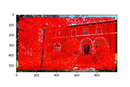
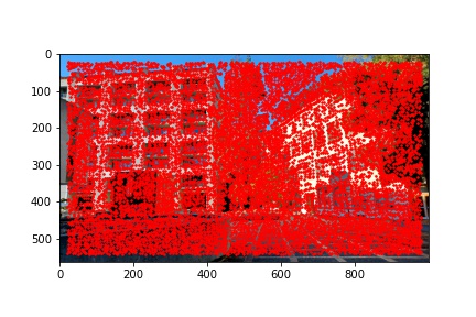
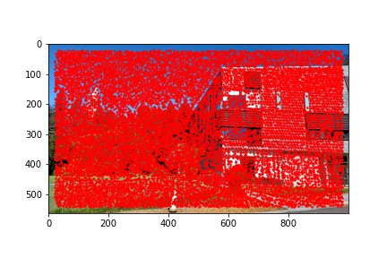
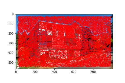
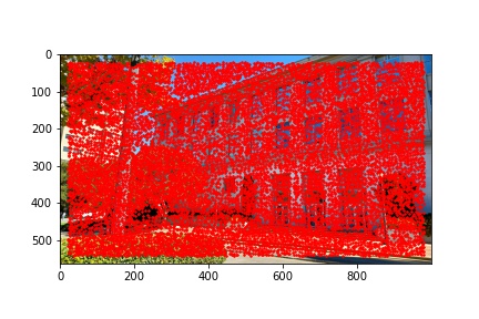
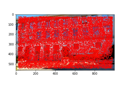
To detect potential correspondence points in an image, in the way of corners, we used the Harris corner detection algorithm. My implementation uses the provided get_harris_corners method provided in harris.py in order to detect all potential corner features in the image. As discussed in class, the intuition behind corner detection is to pass a small window over the image and for each central position, determine whether shifting the window in all directions shows a change in both the x and y derivatives of the window. We are looking for the center dip in the derivative view of the window rather than a valley (corresponding to a line rather than a point) or a plateau (which has neither a corner nor a line). Using these basic principles, we can identify potential corner candidates within an image.
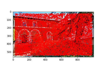
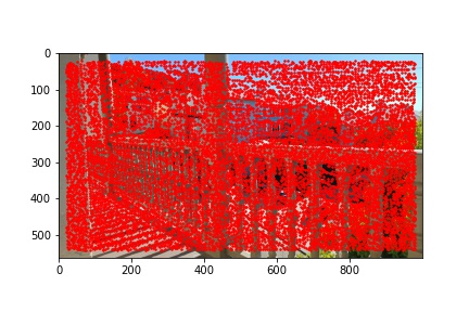
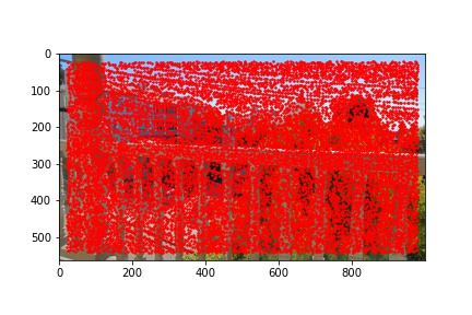
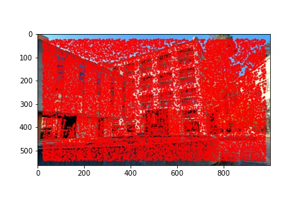
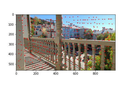
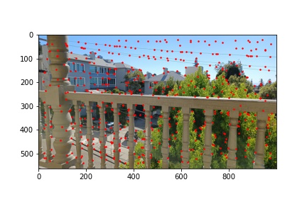
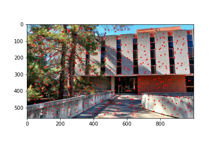
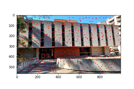
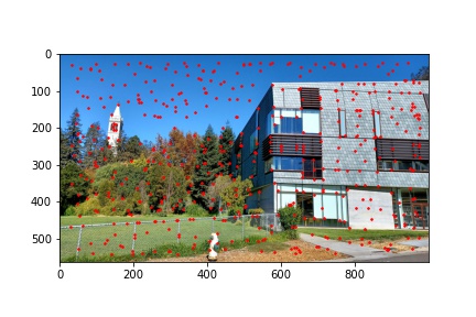
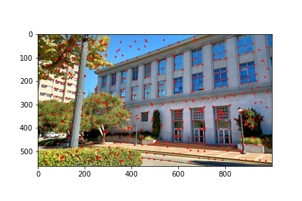
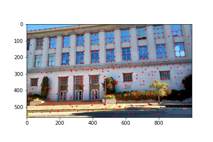
I did notice that there were a lot (really a lot) of detected corners in the image, some of which did not look like corners which is why using the Harris corner detection algorithm alone is not sufficient to compute the homography transformation matrix and additional filtering steps are required. Below are the outputted detected Harris corners in red for each of the images used to produce a mosaic.
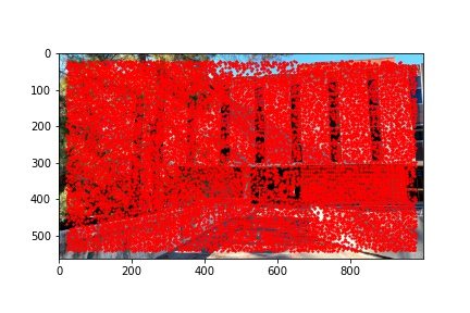
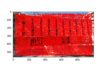
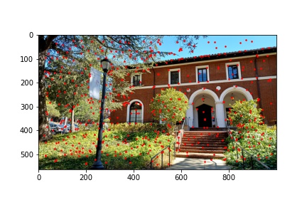
The adaptive non-maximal suppression (ANMS) algorithm allows us to reduce the number of detected corners to 500, or any other specified number but I use 500, which minimizes computing overhead down the line when extracting and matching features for each detected corner. The ANMS algorithm allows us to keep strong detected corners while discarded weaker detected corners all while offering a well-distributed set of corners across the image (rather than ending up having corners clustered only around very sharp points as would be the case if we naively took the top 500 strongest feature corners returned by the Harris corner detector).
I implemented the ANMS algorithm by iterating over every detected corner returned by the Harris corner function and minding the minimum distance between that point and any other detected point which meets the criteria that the other point’s corner strength, multiplied by 0.9, is greater than the corner strength of the current point with which we are processing. Finding the minimum distances to the nearest stronger corner feature for every detected corner in the image, we then sort the list on descending distances (so the first element will have the highest distance and the last element will have the smallest distance) and select the first 500 points from the sorted list of points by descending distances. The ANMS algorithm works well at keeping strong corners while also finding those strong corners in a much more evenly distributed space across the image. The output of the ANMS algorithm for each image to be computed into a mosaic is shown below and the reduction of detected corners, along with their good distribution across the image, is immediately noticeable when compared to the previous images with just the raw detected corners shown.


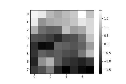
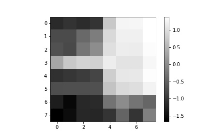
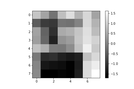
The next step after running the ANMS algorithm to filter out the number of corners detected to the best, well distributed, 500 corner points is to extract feature descriptors for each of the 500 points. This is done by obtaining an axis-aligned 40x40 window patch around each detected corner, the point defining the corner centered within the patch. That 40x40 patch is then down sampled to an 8x8 patch that also undergoes gain normalization. The normalization process is done by subtracting each pixel value in the 8x8 patch with the patch’s mean value and then dividing that difference with the standard deviation of the path. We start with a 40x40 window and down sample in order to extract more information from the surrounding pixels of each detected corner and more robustly complete the next step of matching features between the two images. After all, in an extreme example of only using the pixel intensity at the corner coordinates, the odds of having more than one corner match in the other image with the first image’s corner are very high. Using the 40x40 window and down sampling allows us to more uniquely (though not perfectly) match feature descriptors and get good corner pairings between images. Some examples of 8x8 feature descriptors are displayed below.
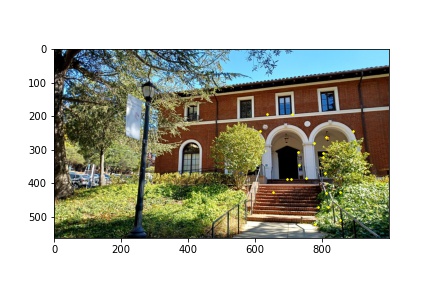
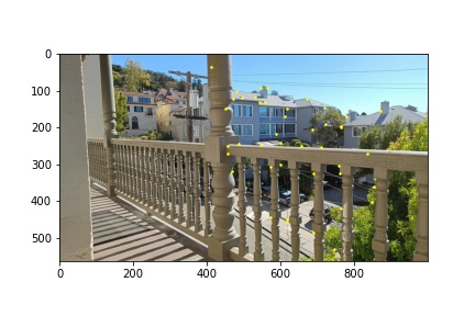
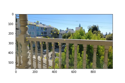
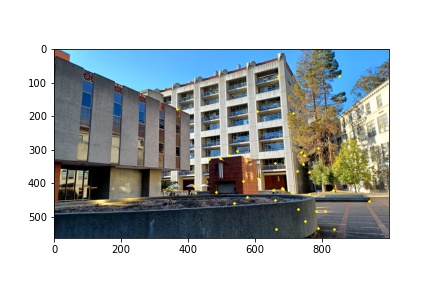
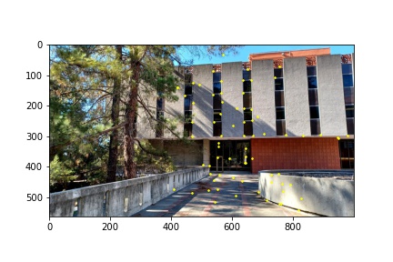
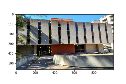
Now that we have 8x8 feature descriptors for each pertinent corner in the images, we perform feature matching using Lowe’s thresholding. I implement this feature matching algorithm by computing the sum-squared difference (SSD) for every feature in one image compared to every feature in the other image. I then sort the returned pairings by increasing SSD so that the first element in the list has the smallest SSD and the second element in the list has the second-smallest SSD value. This is done for every feature in the first image (so the first feature in image 1 has an SSD computed with pairings to every feature in image 2, then the sort is applied to the returned SSDs. Next, the second feature in image 1 has an SSD computed with pairings to every feature in image 2, then the sort is applied to this list of returned SSDs, and so on). I then use Lowe’s threshold to determine whether a pairing is indeed a match by taking the ratio between the smallest SSD and the second smallest SSD in each list and making sure that the ratio is less than 0.3. If this condition is met, meaning that the difference between the best pairing and the second-best pairing is significant enough that we can say with some confidence that the best pairing is a feature match, then we add the feature pair to our list of matches. Below are the outputted feature-matched corners in yellow for each image used to produce a mosaic.

Now that we have feature-matched descriptors, and a more refined corner point selection from which to compute our homography, there is but one more step to complete, further filtering our identified correspondence points. There is still a possibility that a wrong pairing was made in the previous section, resulting in an outlier pairing that would wreak havoc to our homography transformation matrix if we were to compute it using all of the correspondence points thus found. This is where the RANSAC algorithm comes into play, selecting only the correspondence points that match with the other image.
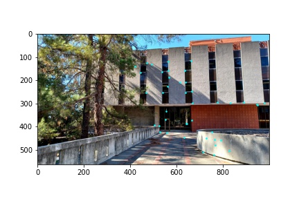
In my implementation, the RANSAC algorithm runs for 1000 iterations and has an error threshold of less than one pixel. On each iteration, four points from those identified as feature matches are randomly selected and a homography transformation matrix is computed on those four points. I then use the transformation matrix on the feature-matched coordinates of the appropriate image and check to see if the transformed coordinates match their true coordinate counterparts in the other image. If they do, then those coordinates are inliers and are added to an inlier list (which is created anew for every iteration). Once all the inliers have been found, I compare to see whether the current set of inliers is greater than the previous highest set of inliers found in a previous iteration of the algorithm. If this iteration’s set is bigger, then the global variables that store the best set of inliers and the homography transformation used to check for inliers are reassigned to this iteration’s inlier set and homography transformation matrix. Otherwise, the function continues to its next iteration. Eventually, by chance, we will come across the homography that has the greatest number of inliers, with errors using the homography transformation matrix of less than 1 pixel. These inlier coordinates are what we use to now recompute the homography, with more than just four points so that we can also get some of the benefits of least squares when computing the homography, and use it to perform the image warps and produce the mosaics shown in the next section. Below though are the final correspondence points identified in the images shown in cyan.


Now that we have computed our homography transformation matrix given a set of automatically detected correspondence points, we proceed with the same steps as from part A above to warp and blend the images together to produce a mosaic.
To briefly overview the process, I begin by determining the transformed pixel coordinates from applying the homography transformation on the corners of the image. This gives me an idea of how much padding I should add to the left, right, top and bottom parts of the images in order to compute the homography without losing details from the image (due to coordinates being transformed off the canvas). After determining the paddings, and producing masks that identify where each image lies on the mosaic canvas, I proceed to perform the warp using the previously computed homography transformation matrix. Since we are padding the images, I modified the warping method to first transform the pixel coordinates into the previous, non-padded coordinates with a simple translation matrix, then apply the inverse homography (to perform inverse sampling), and then apply the inverse translation matrix to convert the coordinates back into the coordinate space of the mosaic canvas. I found this solution to be more intelligible than using cv2’s remap function. The masks for each image are also warped, since these masks are used to produce the final image blend.
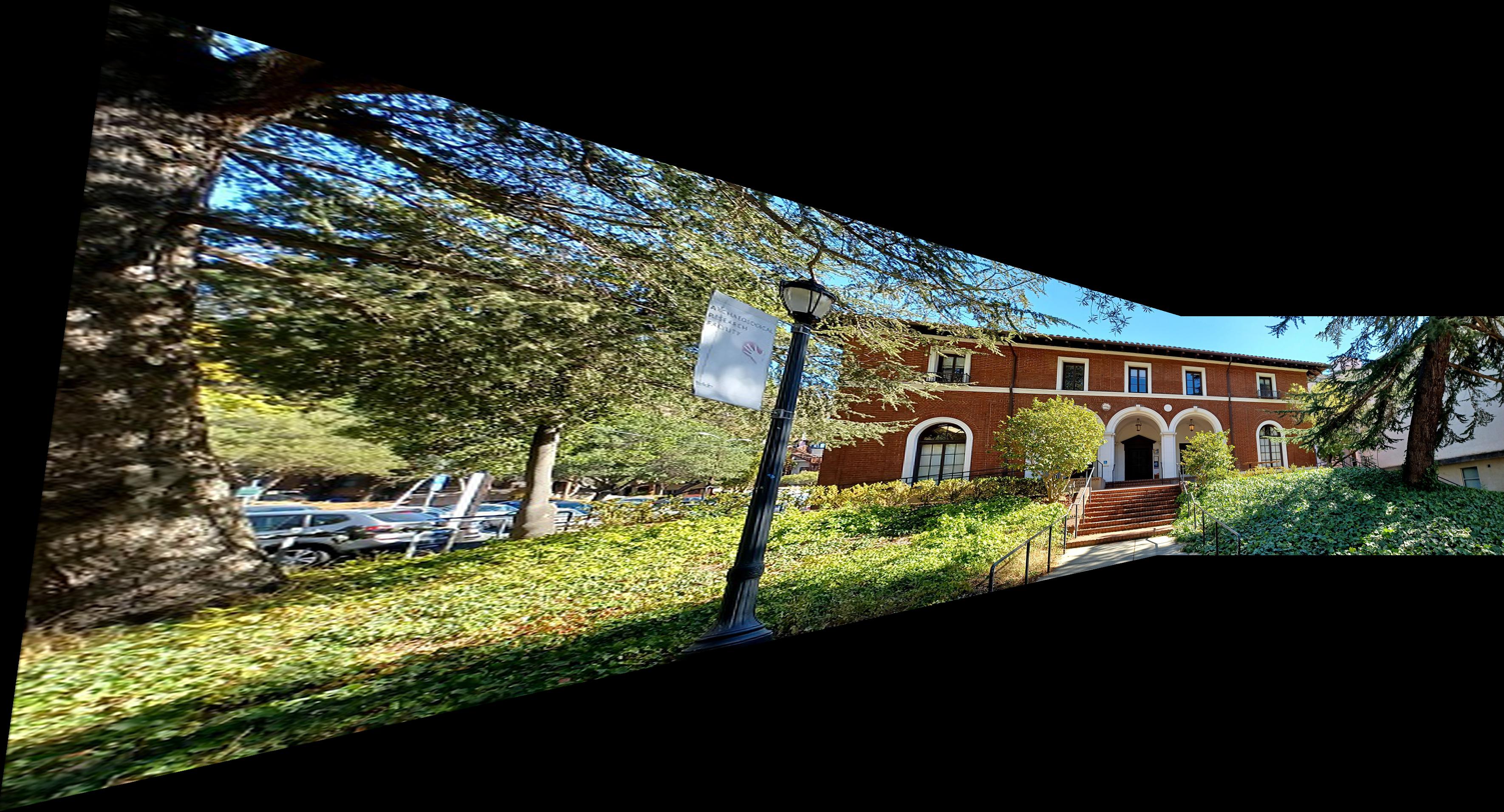
The image blending process consists of identifying the intersecting pixels between two image masks, then producing a gradient on that intersection patch as to blend the color transition between the two images and make the image stitching seams less visible. More detailed descriptions of how the homography is computed, warp is performed, and blending is achieved are available in the part A write-up above since these functions used in part B of this project are nearly identical to the ones used in part A. The modifications made were some method signatures to accommodate additional arguments but the algorithms are the same. Below are the final image mosaics that were produced using automatic feature detection and their manual stitching result counterparts are also viewable for comparison.
Overall, it is quite obvious that the automatic stitching algorithm produces much sharper mosaics than the manual stitching which is to be expected since manually identifying corner features in an image cannot be pixel precise every time while the automatic stitching algorithm is designed to be pixel precise.
Definitely the process for automatically detecting correspondence points with which to perform image stitching was the coolest part of this project. It was interesting to learn how the Harris corner detection algorithm worked and the ANMS algorithm was also really cool to get good distributed corners on an image, but I was most impressed with the simplistic power of RANSAC to remove outliers from the filtered coordinates with only 1000 iterations (though my points upon inspection contained very few outliers prior to running RANSAC which allowed for fewer iterations to be required). But knowing that as long as at least 50 percent of the identified points are good pairings, increasing the number of iterations will filter out even very bad pre-matching algorithms. Really, the whole process of automatic corner detection, feature descriptions, and automatic stitching of images to produce mosaics was probably the most fascinating (though at times painful to debug) projects I have done.