Part A: Image Warping and Mosaicing

Overview

This project utilizes projective transformations to stitch together images taken from the same viewpoint to form a mosaic or panaroma.

Shoot the Pictures

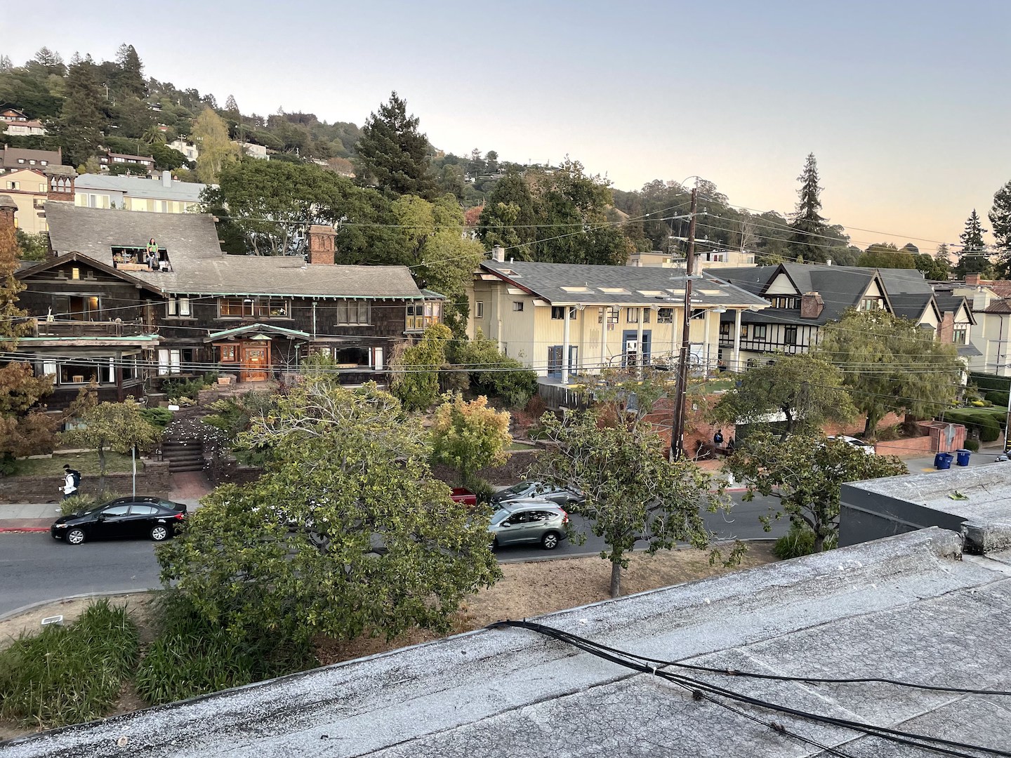
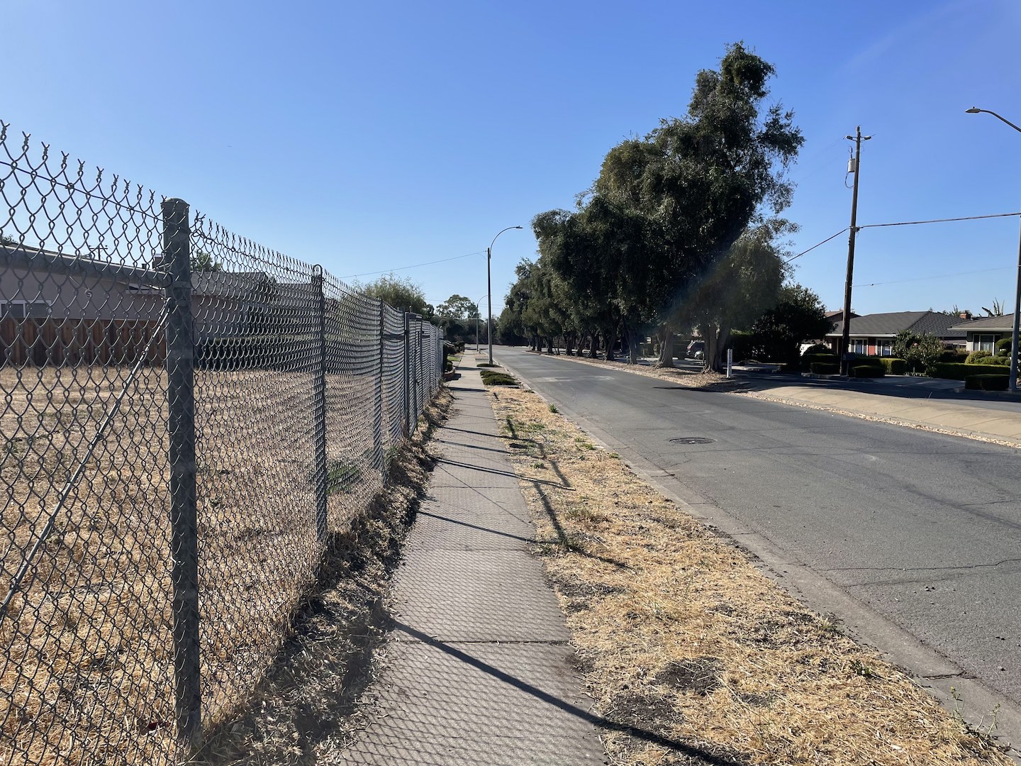
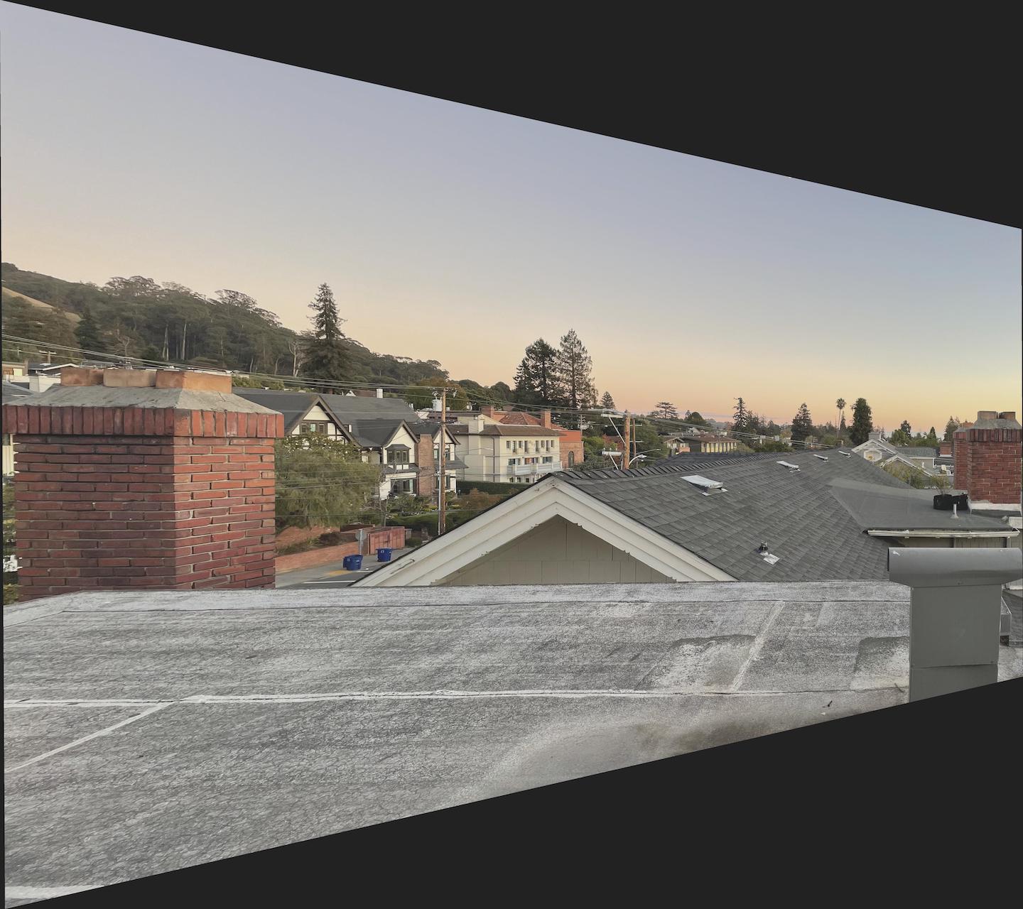
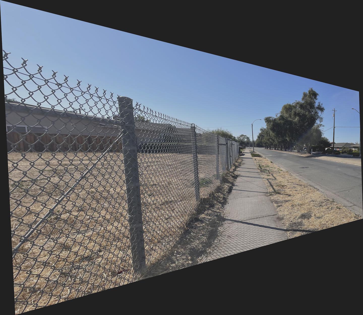
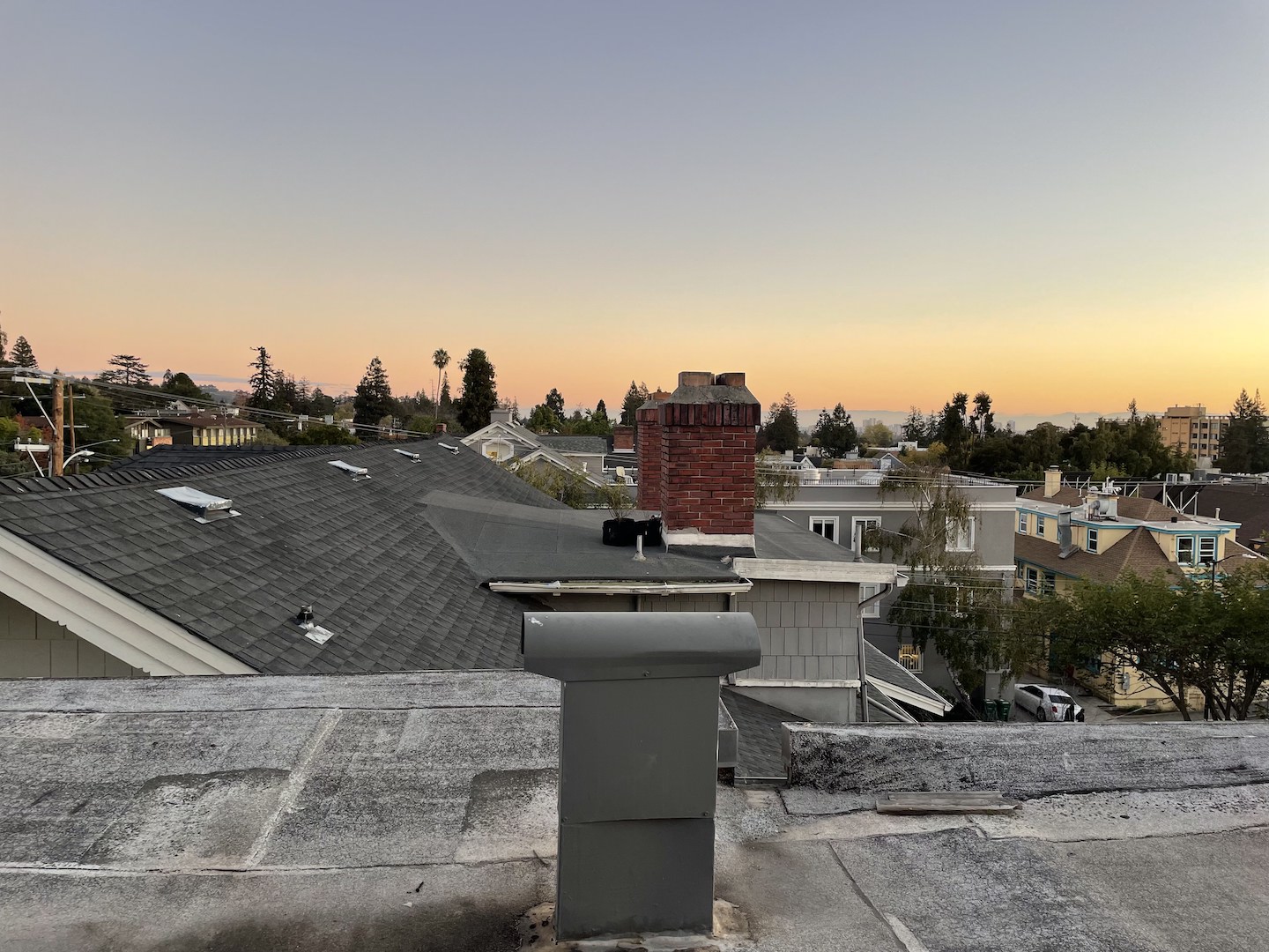
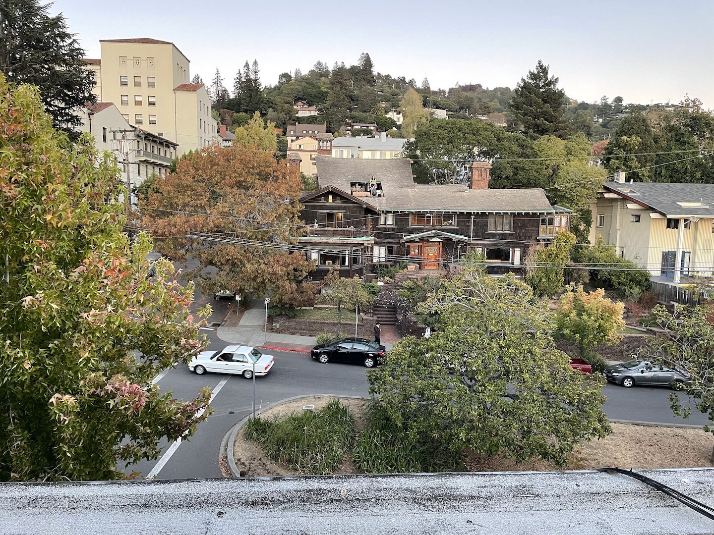
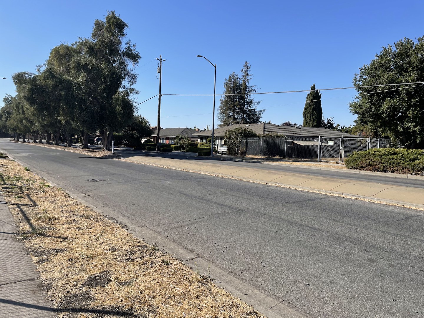
Here are various scenes taken by me from the same viewpoint at 2 different angles.

Recovering Homographies

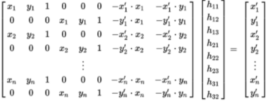
To recover the homography transformation that will allow the images to be in the same plane, I transformed selected points from each image and set up linear equations for least squares in the form Ax = b. Below is an image that exactly describes how the points p1 and p2 are converted into an A and b matrix then passed into the np.linalg.lstsq function. Since there are only 8 dof, our returned result will have the shape (8,1). To convert this to the transformation matrix that we know and love, I appended a 1 and reshaped the vector into a 3x3 matrix.

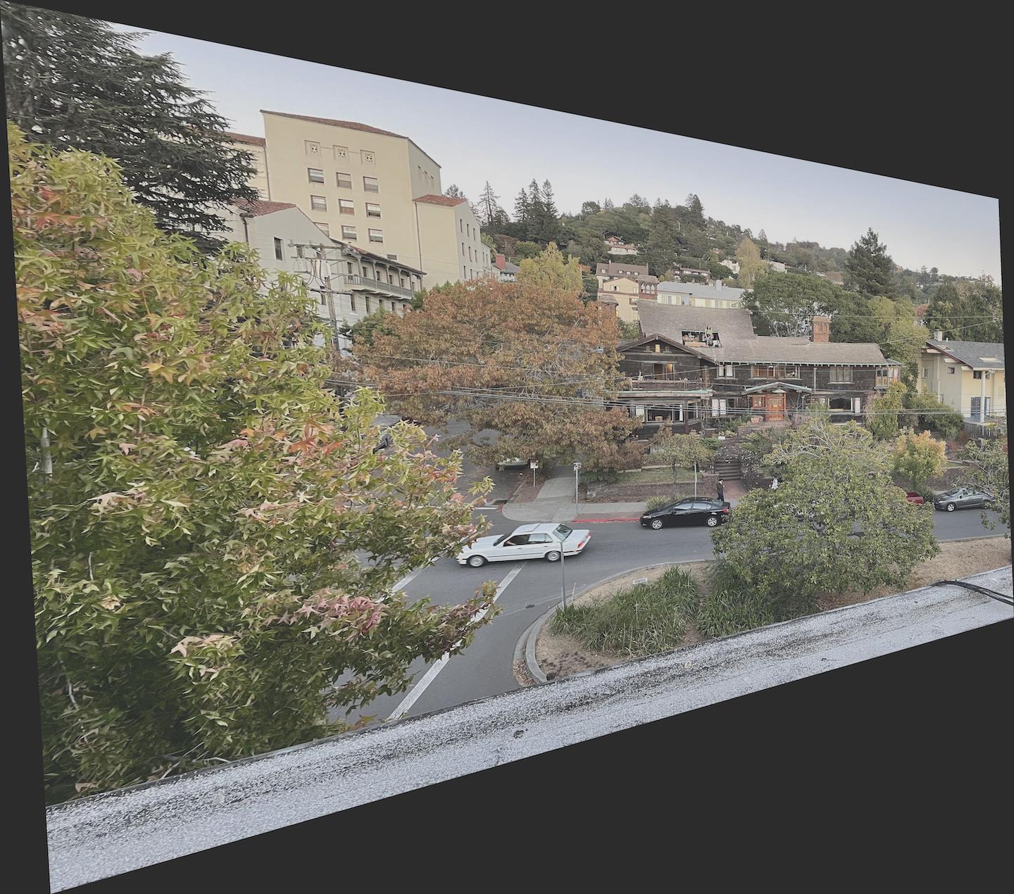
Warp the Images

Using a similar process as Project 3 and the RectBivariateSpline function, I used the homography matrix from the previous to set up an inverse warp from the original image to the warped image. One caveat is the new bounding box post-warp. This was harder to determine as previously we had an exact triangle to triangle mapping. To determine the bounding box, I warped the corners of the original image and calculated the max range for rows and columns, making sure to translate the image when populating index values as some were negative and the polygon would ignore negative values. These values were eventually translated back when plugging into the inverse warp function. The results of the warp are below.

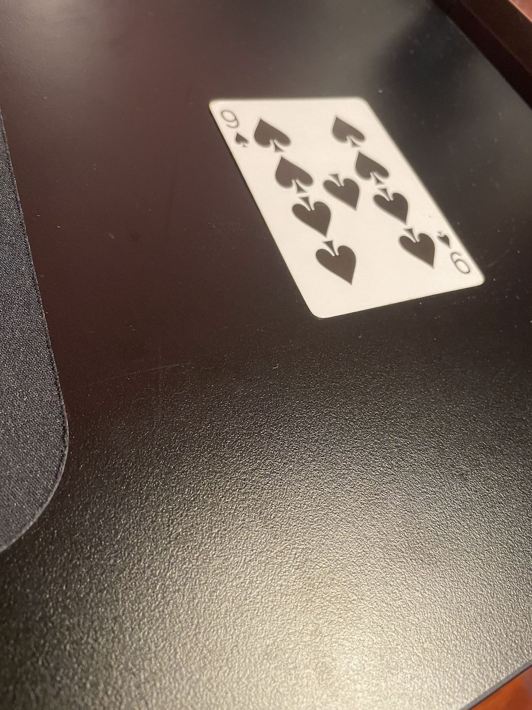
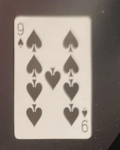
Image Rectification

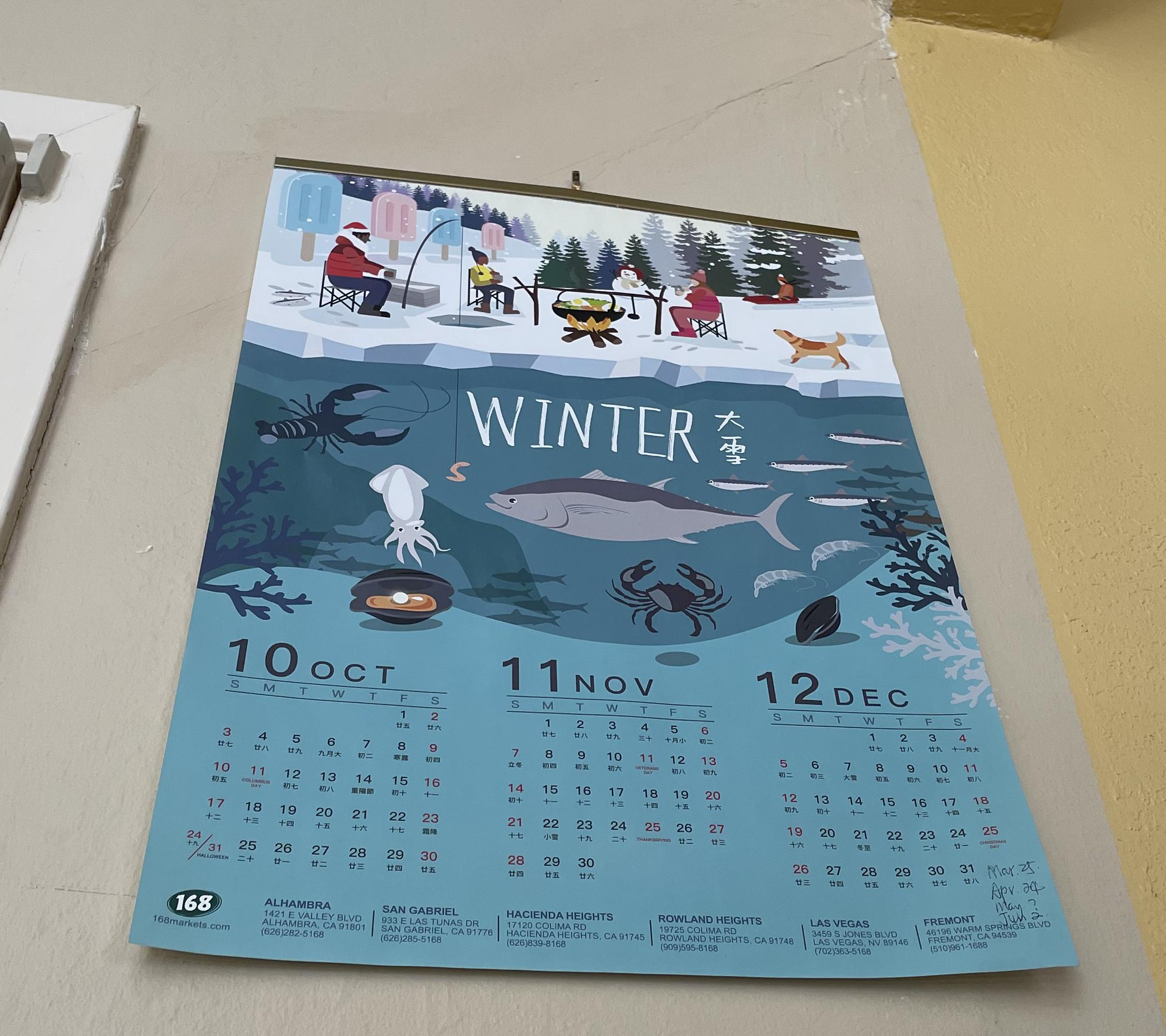
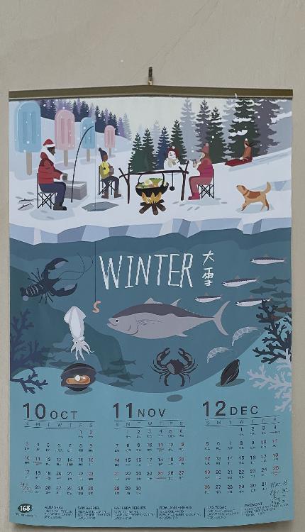
For this portion of the project, I used the warp function from the previous part to test my homographies. I took a picture of a poster and playing card at off angles and used the warp function to create a top-down view of the objects. This was done by selecting points on the corners of the poster and playing card and mapping these points to a flat plane with corners that mimicked their rectangular dimensions. The results are below.

Note: The card itself was blurred in the upper right corner due to focusing and is thus reflected in the top-down image. As the blur is exaggerated due to a lack of information in that area.

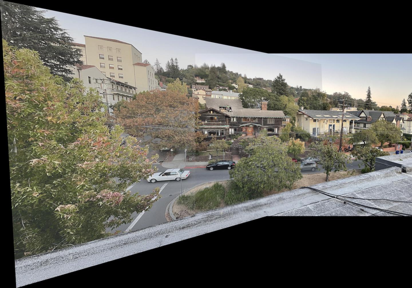
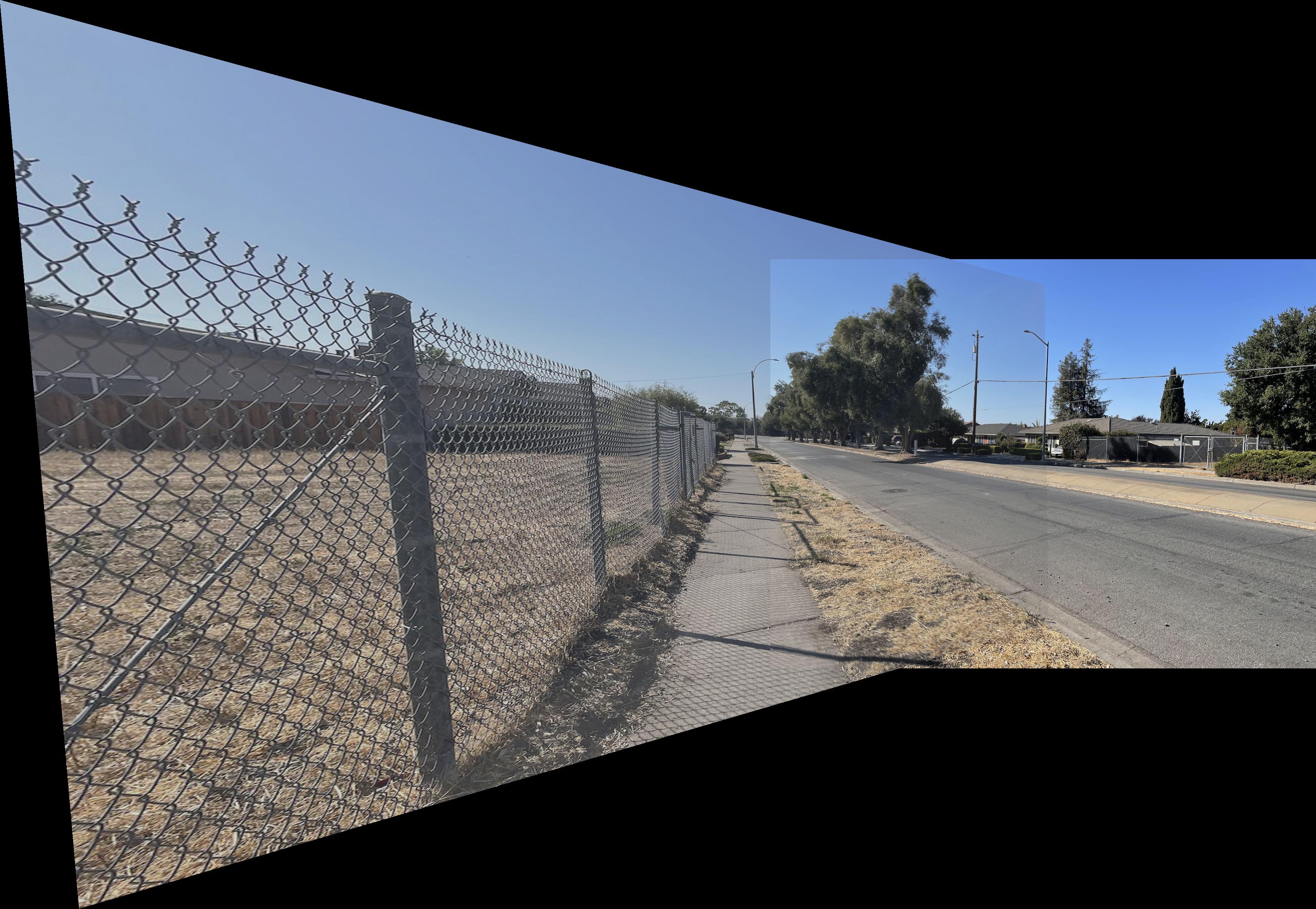
Blend the images into a mosaic

To blend the images, I shifted the second image such that the selected feature points were in the same location. To do this, a new image array was created to accomodate the increase in image size due to the shift. I then created an alpha layer using the warped polygon and the secondary image. The warped-polygon-only pixels were set to pixel value 1 while the second image-only pixels were set to 0. The overlapping area is set to 0.5. This layer is then multiplied by the warped image and 1-alpha * second image. This effectively averages the overlapping area and creates a stitched image. Notice that since laplacian stacks were not used, the blending and seams are noticeable. One thing that I noticed was that shrubbery and trees were noticeably harder to align as feature points generaly ignored that area (hard to consistently label those locations). The results of 3 stitching scenes are displayed below.

Overall, the most interesting I learned from is once again the importance of feature selection. The points that were chosen ultimately aligned the objects they were outlining (i.e. buildings, cars, poles). However, objects that were more difficult to align such as trees and shrubbery (which may also have moved due to wind conditions) ultimately remained blurry and unfocused.

Part B: Feature Matching for Autostitching

Overview

This project utilizes harris points, lowe's trick, nearest neighbor, adaptive non-maximal suppresion, and RANSAC to detect points of interest in images, isolate high probability pairings and compute a homography based on those pairs. This aims to build on top of the previous part of the project where the main hassle was selecting points between pairs of images. This project automates this process to achieve a comparable or even better stitching experience.

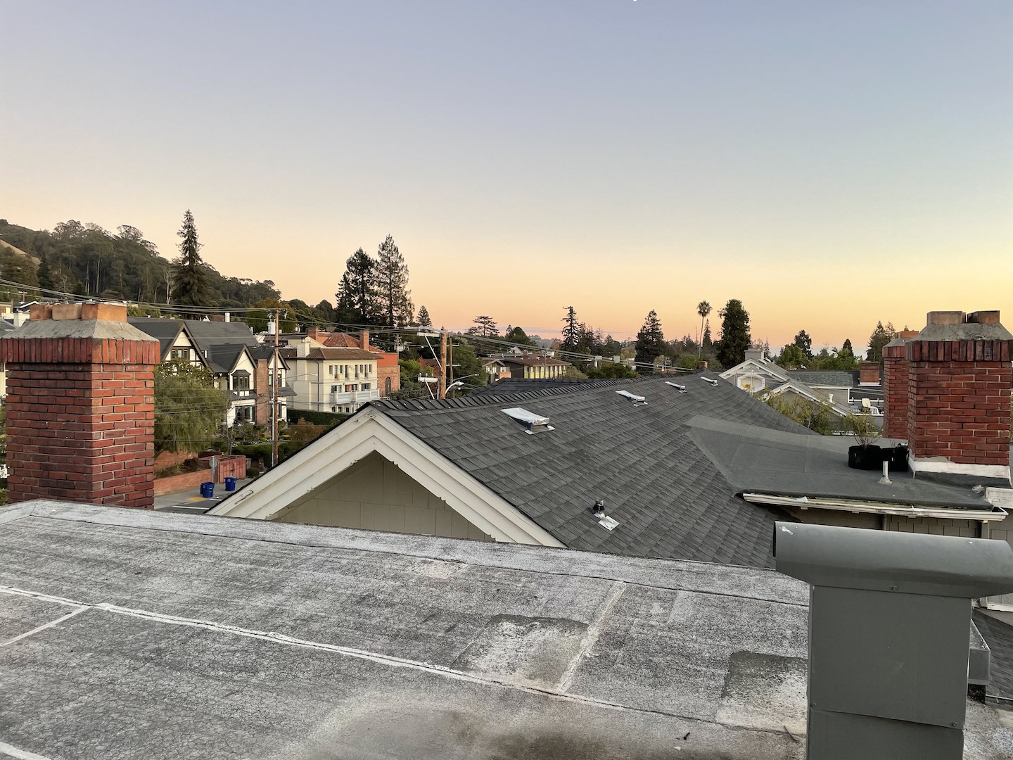
Images

Here are various scenes taken by me from the same viewpoint at 2 different angles (same images used in the previous part of the project). The sections of this project will be demonstrated using the Apartment Roof images. Similar processes were used to derive the automatic stitching of the other 2 sets of images.

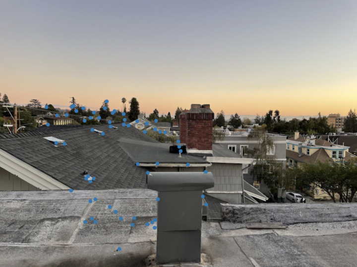
Harris Interest Point Detector

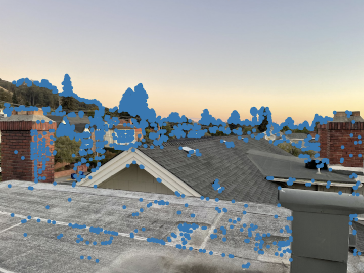
To detect the Harris Interest Points, I used the provided boilerplate code, mainly the get_harris_corners function to derive a set of interest points. Then, I used the corner strength matrix to filter out some of the less important points. The harris points that we are left with are displayed below.

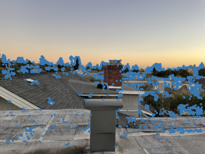
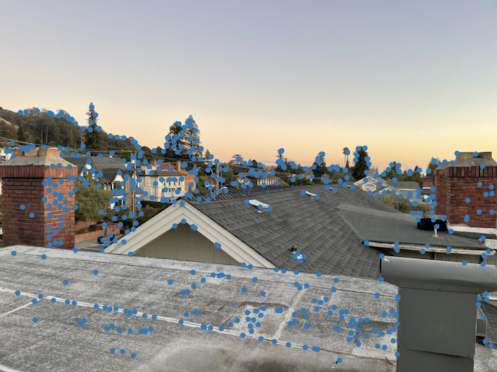
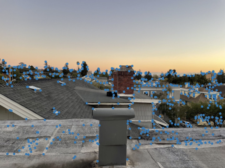
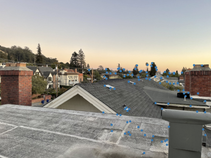
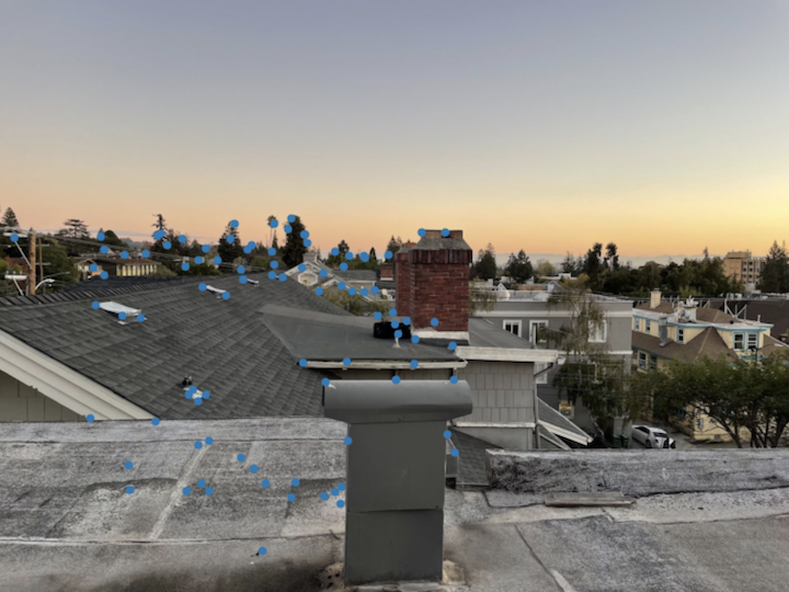
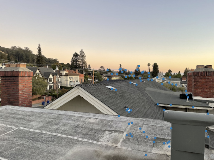
Adaptive Non-maximal Suppression

The main idea of this next step is to eliminate the clumped up nature of the vanilla harris points. To do this, I followed the formula for ri (the minimum suprression radius) to derive ri values for each of the harris points displayed above. These values were then sorted and the top 500 points were retained for further processing. The points remaining after ANMS are displayed below.

Notice: The points in the above images are better spread out while still retaining a good coverage of the key points of interest.

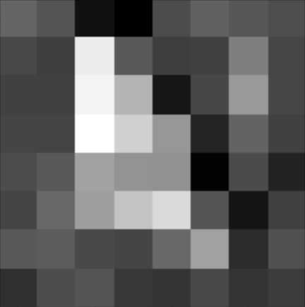
Feature Descriptor Extraction

In this portion of the project, I follow the process mentioned in the paper to derive an 8x8 feature descriptor from a 40x40 pixel field centered around each of the interest points. This pixel field was then downsampled to 8x8 and bias/gain normalized. Below are some random images of these descriptors.

Feature Matching

The next step is to actually take the above features from either image and attempt to pair them as best as possible. Here I used Lowe's trick to identify "goood pairs". By calculating the 2-nearest neighbors in image 2 for each pixel in image 1 and constructing a ratio from the errors, I set a threshold to both prevent a large portion of bad pairings and encourage a large portion of good pairings. The lowe's points are displayed below.

4-Point RANSAC

Once these pairings are established, we further optimize these points to calculate a homography that fits a large portion of these pairs. We employ some randomness here so the results are not always the same. To begin, 4 random points from the previous parts are chosen and a homography is computed from them. This homography is then used to determine a consensus between the other points w/ an error threshold. I compared the predicted image 2 points with the actual image 2 points and eliminated pairs that differed more than the threshold (e = 20). This process was performed for 1000 iterations and the best case result was returned for stitching/blending. The results of these pairs are below.

Notice: The points that are retained correlate nicely in the images.

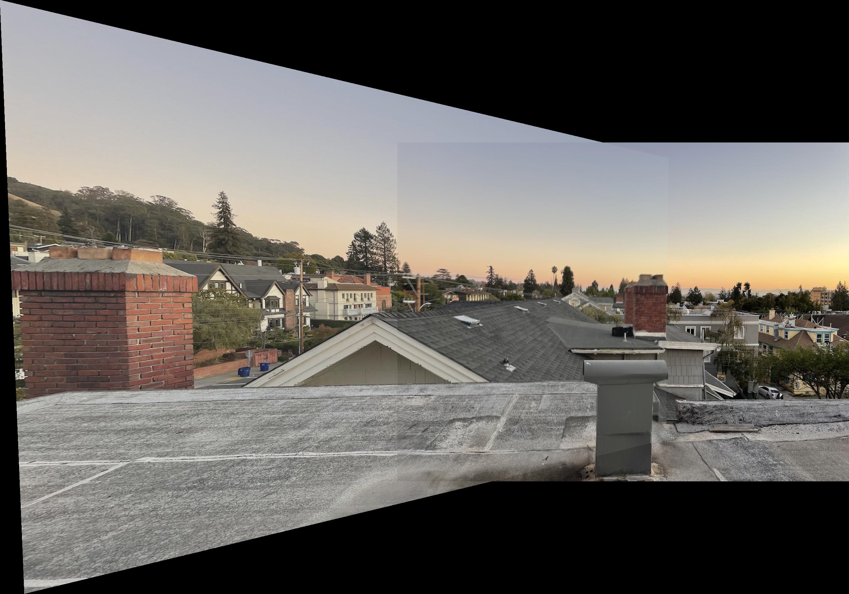
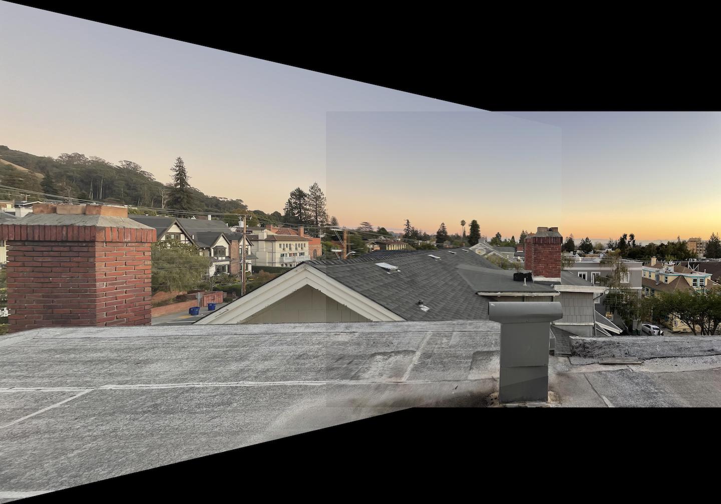
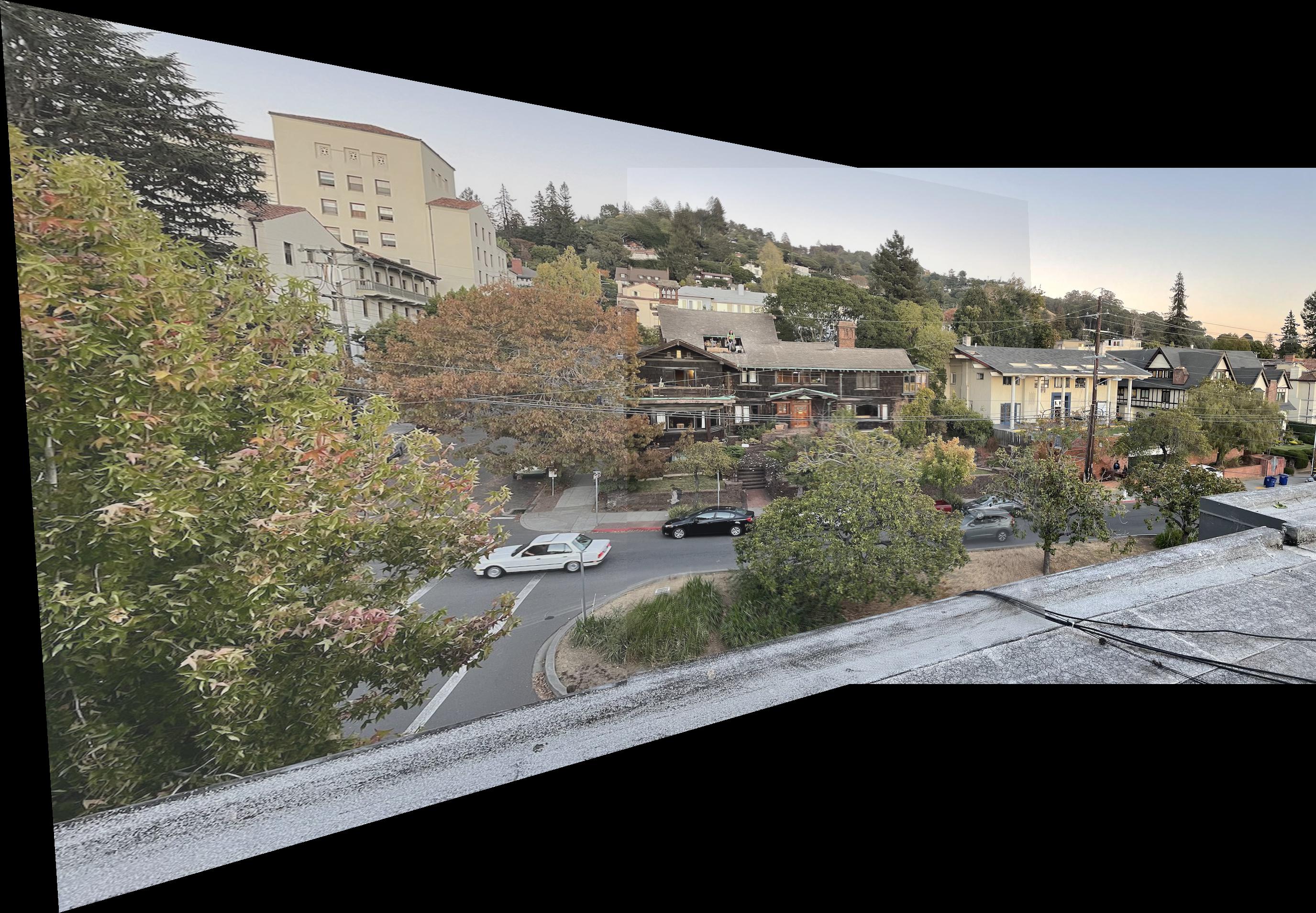
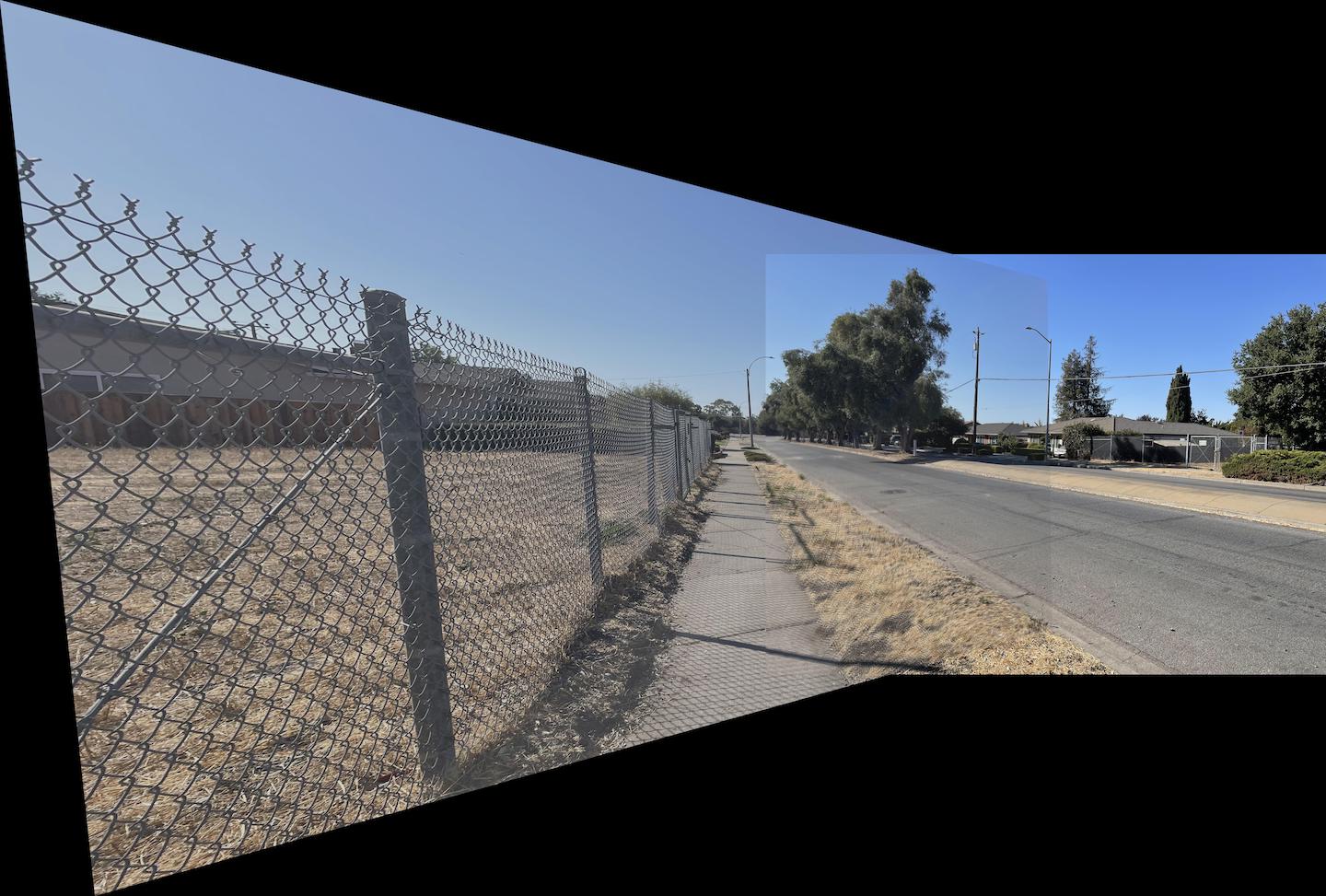
Stitching

The last part computes a least-squares homography from the RANSAC points and applies this to the pair of images. Using the functions for warping and blending from project 4a, these images are then stitched. The results are displayed below and compared to the results from the manual point selection in project 4a.

Notice: Due to the difference in points selected, different parts of the overlapping areas perform differently across the two stitching schemes. More points = more focus and less blurry.

Conclusion

Overall, I found the Lowe's trick the coolest thing from this project. It is just extremely useful in separating the useful points from the noise.