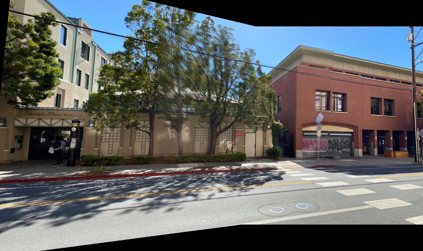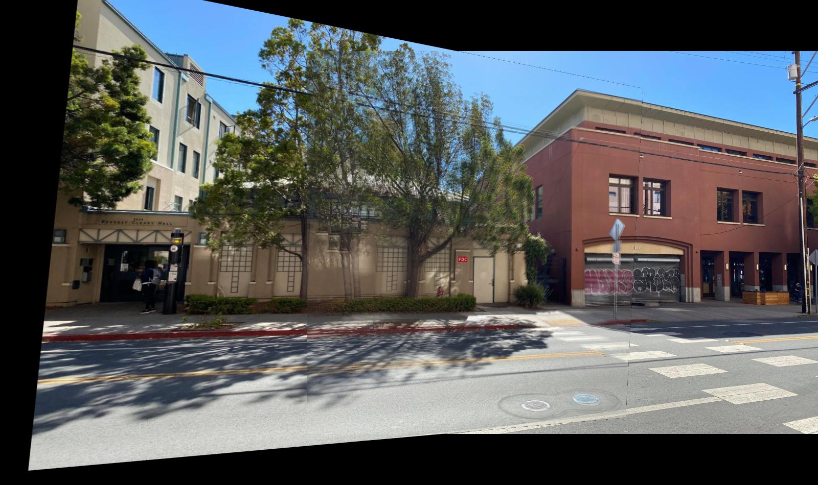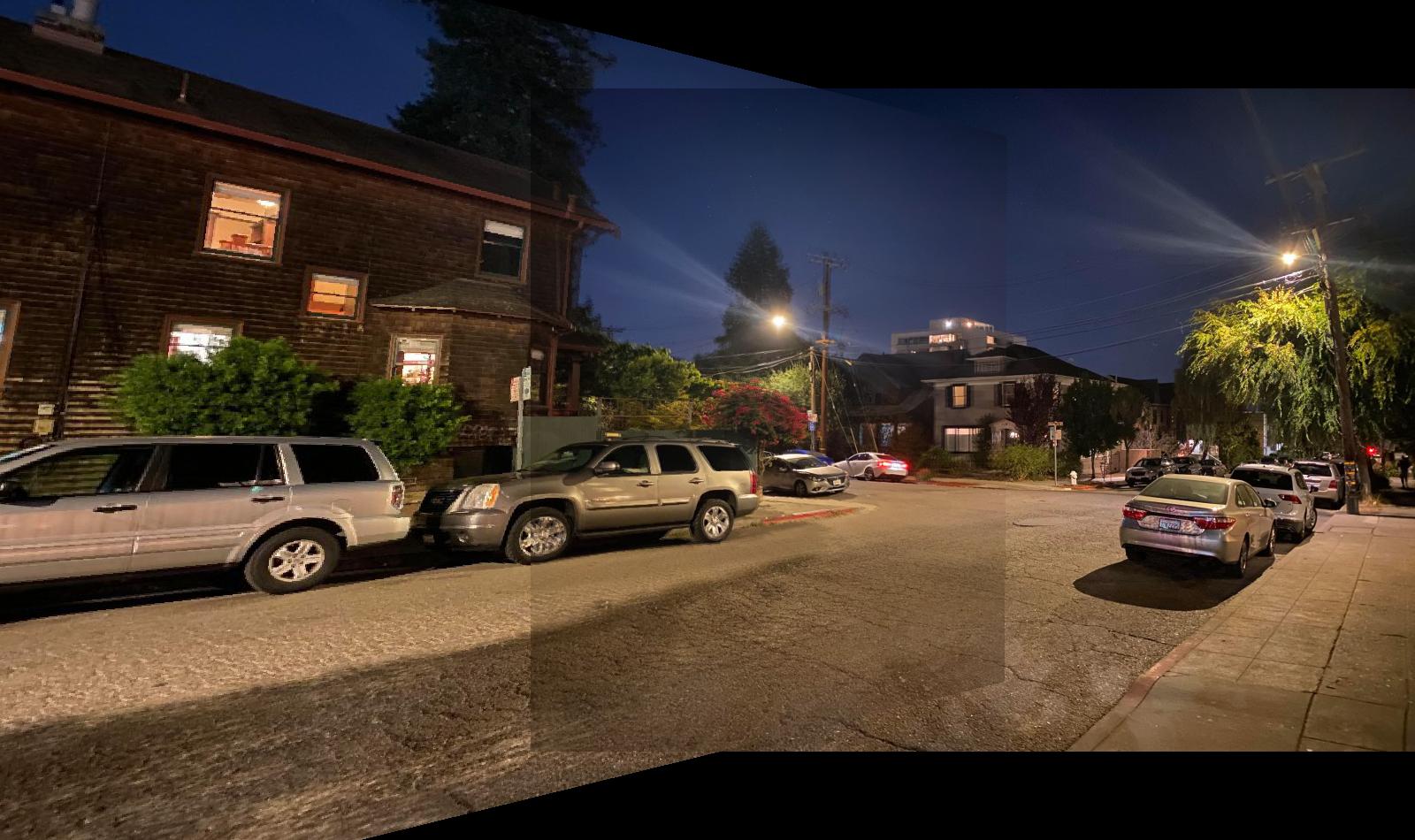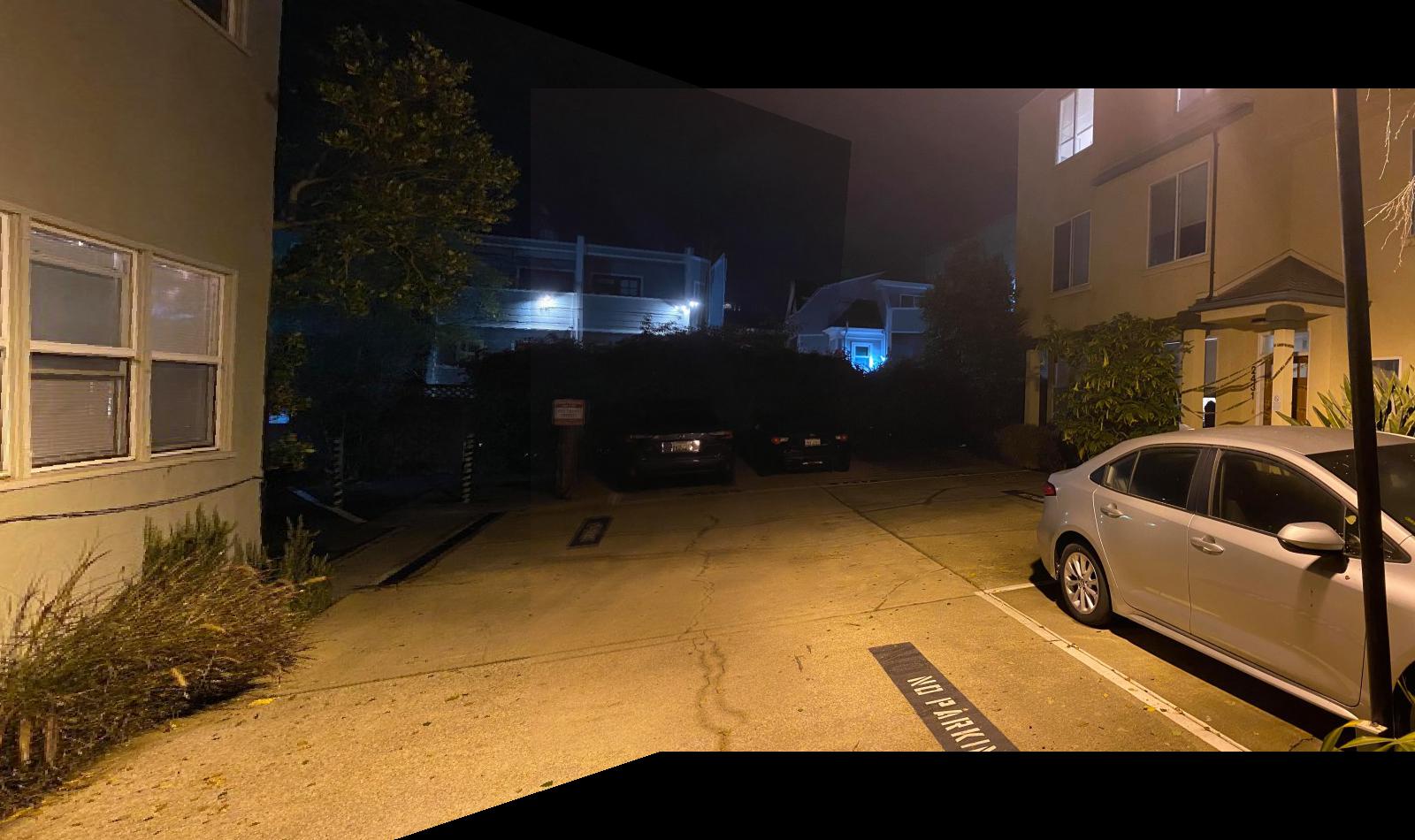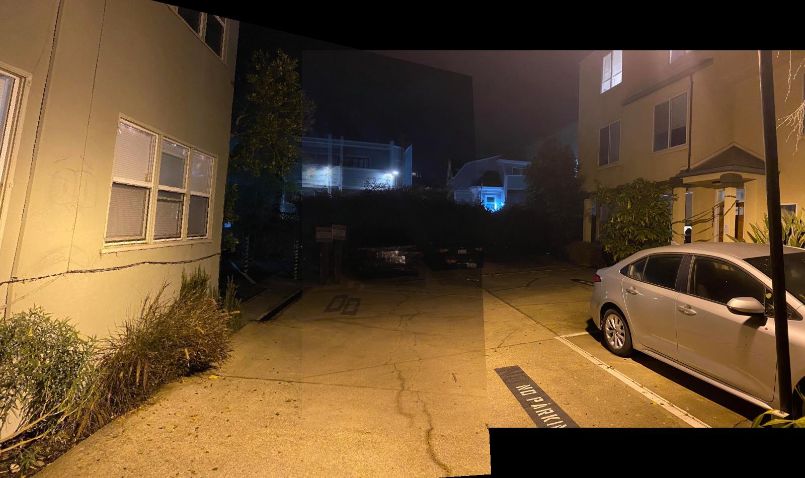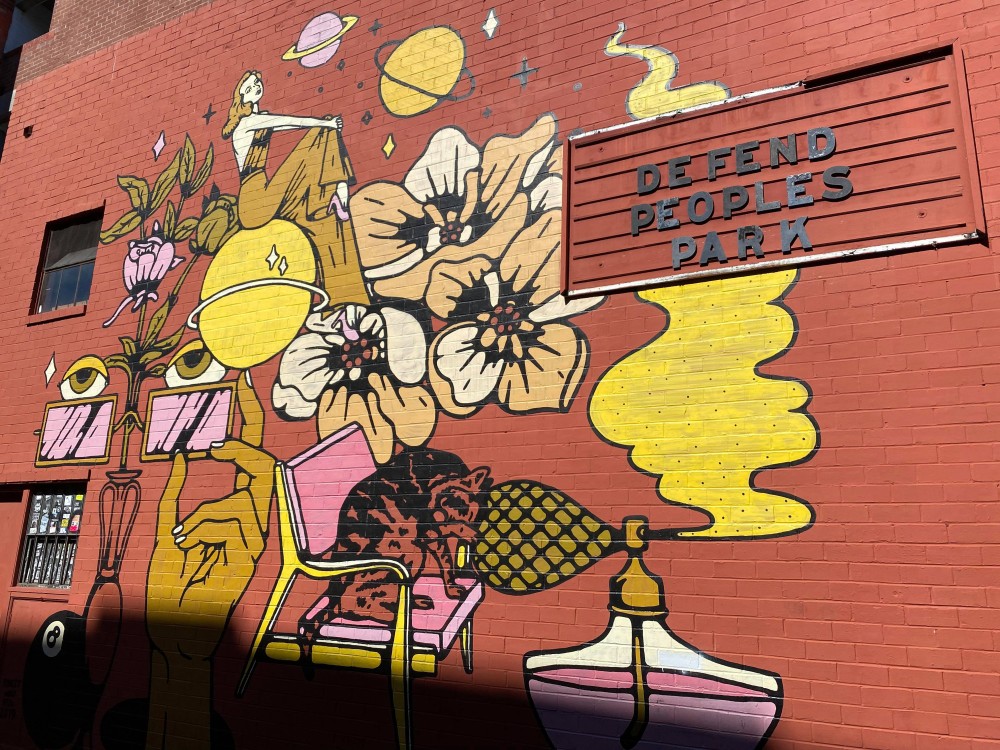
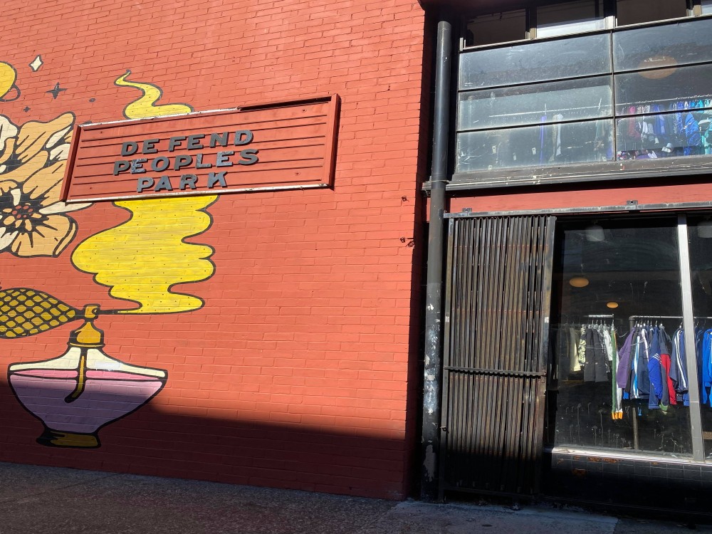
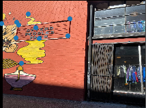
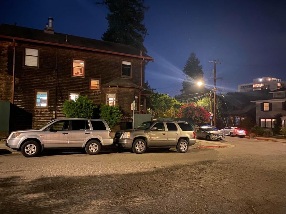
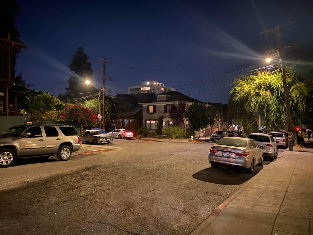
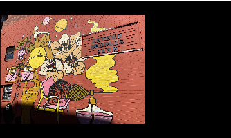
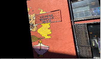
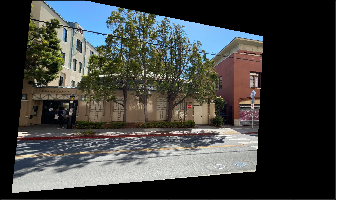
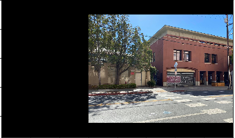
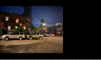
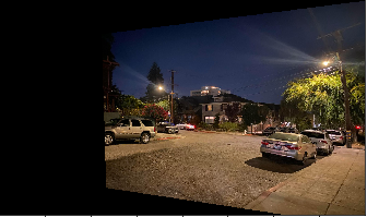
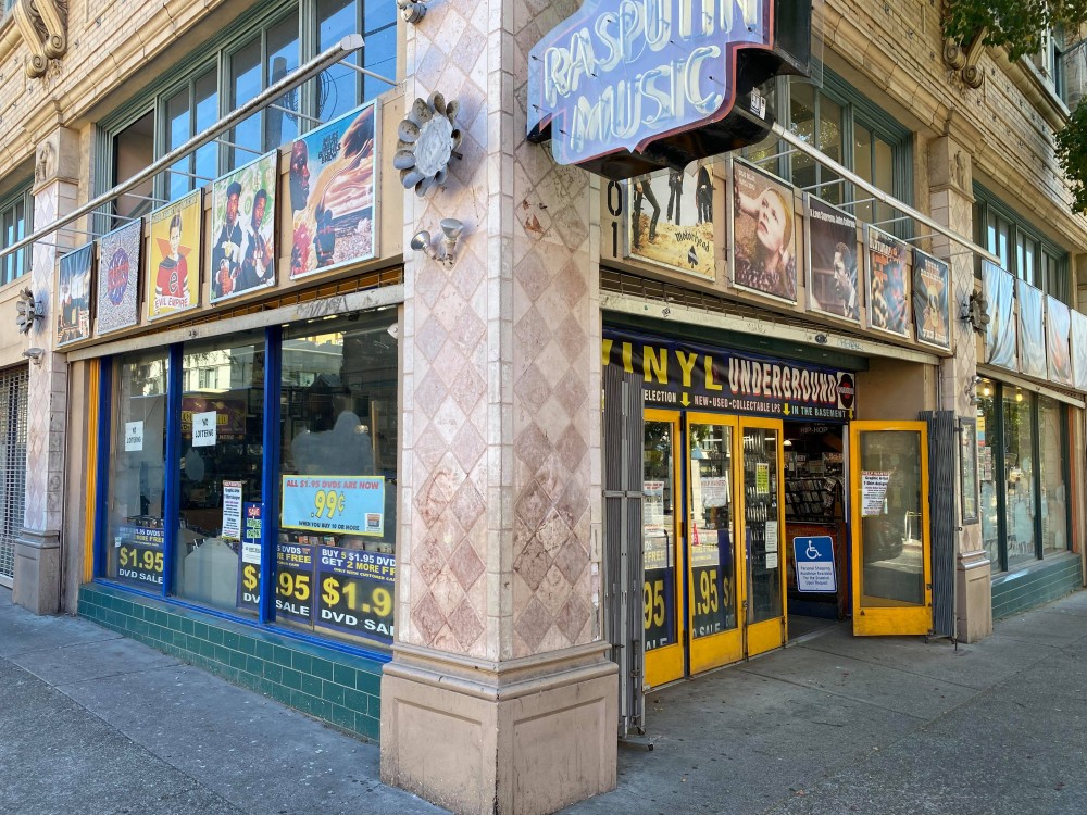
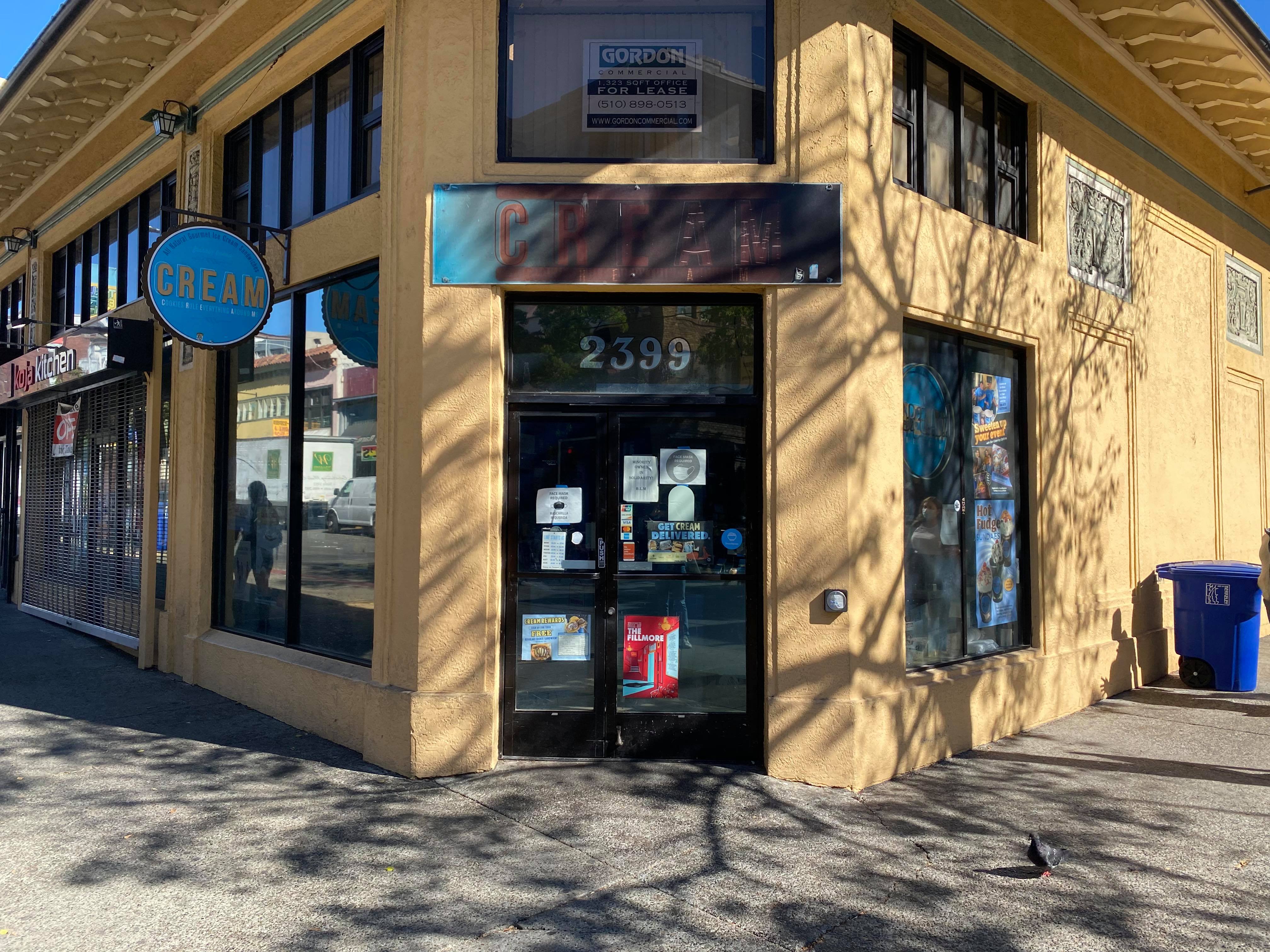
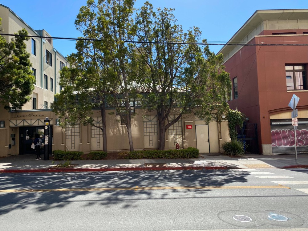
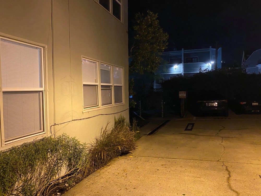
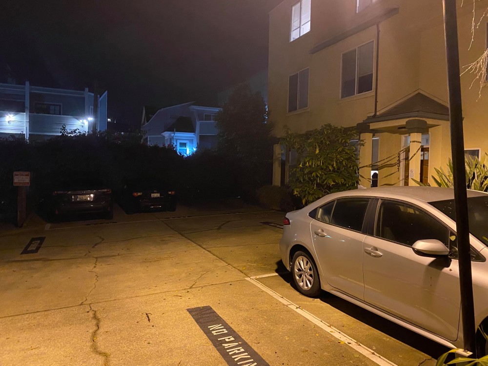
For this step I shot pictures of some murals and streets around Berkeley, and defined 10 corresponding points between pairs of images of the same scene from a different perspective.

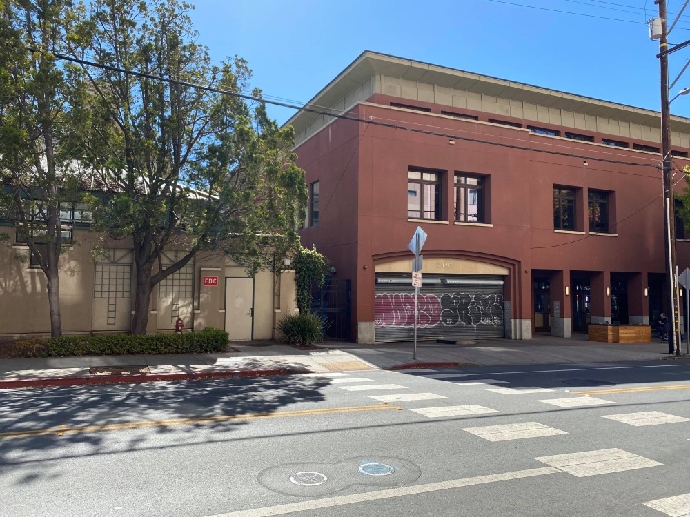
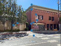
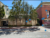
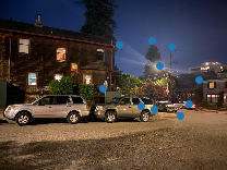
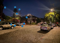
For recovering homographies, we defined the keypoints as shown above. We then used overparameterized least squares in order to try and accurately estimate the homography between the two images that we loaded in the previous section.
This yielded a 3x3 matrix defining a transformation from a set of points in one image to a set of points in another, which we could use to perform the warping for rectifying images and constructing mosaics.
In order to warp the images, we used the homography matrix H we calculated to transform the set of points in a given image into a set of points from which to sample from the image. I used the cv2.remap function in order to sample the transformed points from the original image (I also experimented with using RectBivariateSpline, and had reasonable results, but ran into issues on the borders of images).
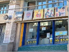
Something else interesting that can be done is rectifying an image to show a planar surface in a frontal-parallel fashion. This was done to validate the warping, with keypoints for the plane corresponding the the four corners of the original image for calculating the homography.

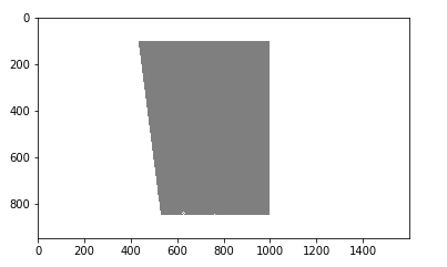
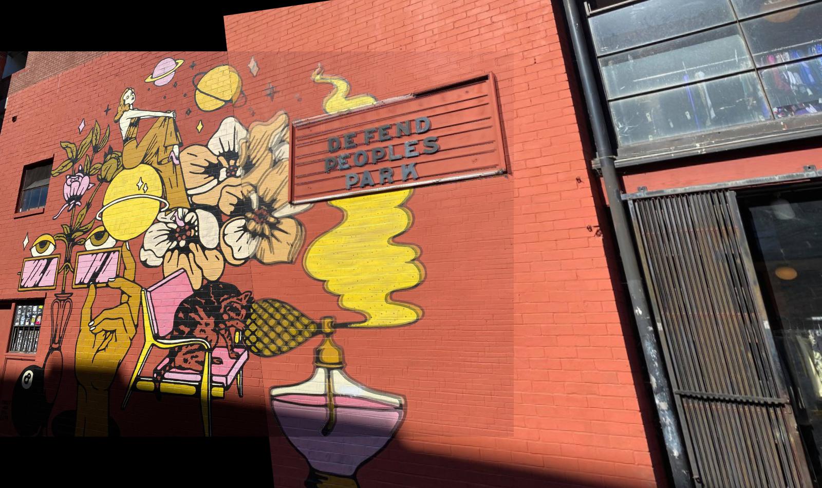
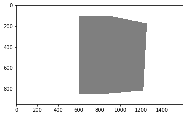
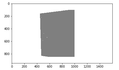
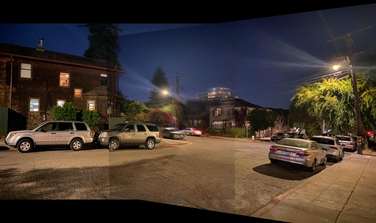
Finally, we blended warped images together into a mosaic, combining them using weighted averaging. I computed a mask of the overlapping region between two images in the mosaic, and set the mask value to be 0.5 in the overlapping region in order to try and best blend the two images together. The value in the mask would have to be updated for any additional image that also overlapped in the same region.

In Part 2 of this project, we attempted to automate the process of picking points for aligning images in order to create a homography between them. The implementation chosen for generating and matching features was based off of the paper "Multi-Image Matching using Multi-Scale Oriented Patches" by Brown et al.
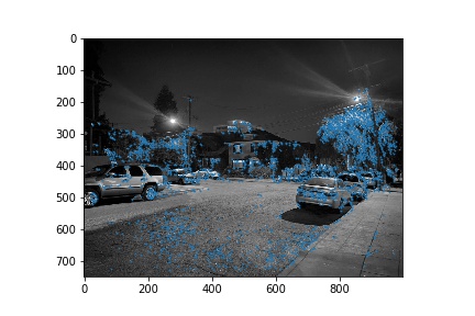
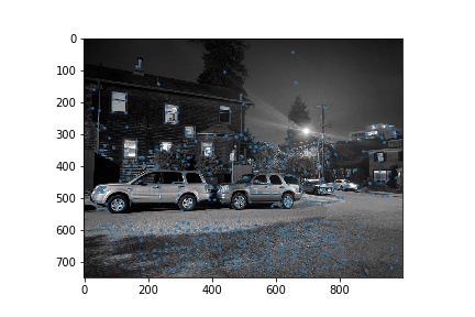
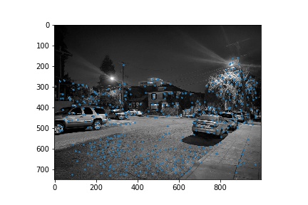
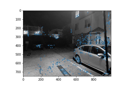
We first used the Harris interest point detection algorithm in order to identify corners that would be good for aligning images with. The results of generating Harris interest points with a relative threshold of 0.05 are shown below for each of the 3 pairs of images used in this next section.


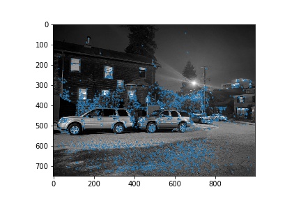
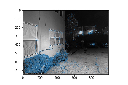

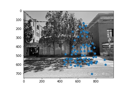
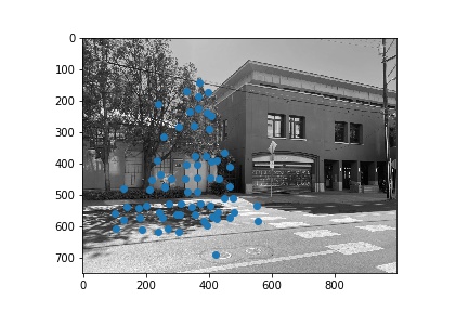
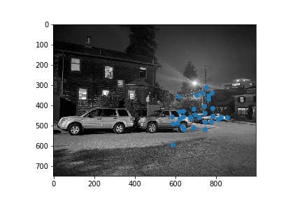
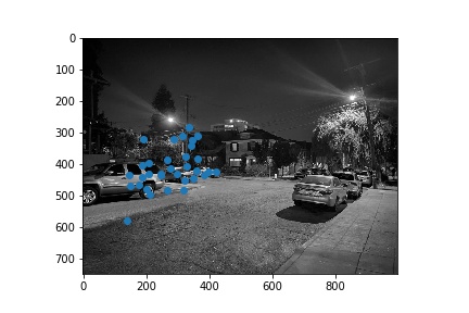
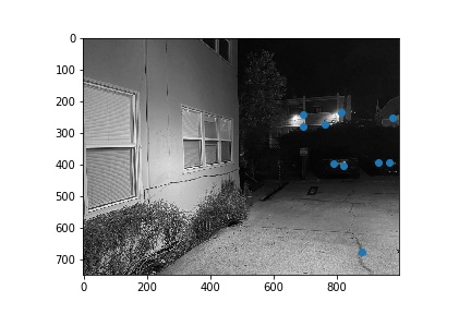
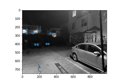
Next, we narrowed down the set of corners selected in the previous section using the Harris point detector using Adaptive Non-Maximal Suppression in order to generate a set of strong points of interest that are spatially distributed well over the image. Using the algorithm as described in Brown et al's paper, we narrowed down the number of interest points to 500 per image. These points are shown below for each image pair.
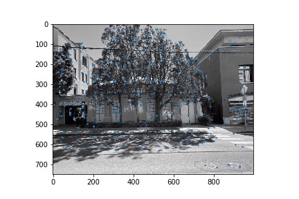
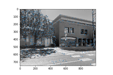

Once we narrowed down our set of corners, we sampled a 40x40 window around each of them, then downsampled that 40x40 window to an 8x8 patch, which was then normalized. Thus, each of the points had a length 64 vector describing the features locally at that point.
Once we extracted our features, we used the sklearn implementation of nearest neighbors in order to get the nearest neighbors in terms of the features to each of the points in our two images. We used the basic approach to Lowe thresholding, by thresholding on the ratio between the first and second nearest neighbors. This gave us a set of features that matched between the two images that we could then use to compute a homography.
Next, once we had a set of matching coordinates between images, we filtered out matches that were not accurate using RANSAC. We set epsilon to have a value of 5, and found the set of indices within the matched pairs that gave the homography that included the most indices as being accurate under the threshold. We then computed H using the pairs corresponding to the inlier indices - after which, we were ready to warp our images to form mosaics again.